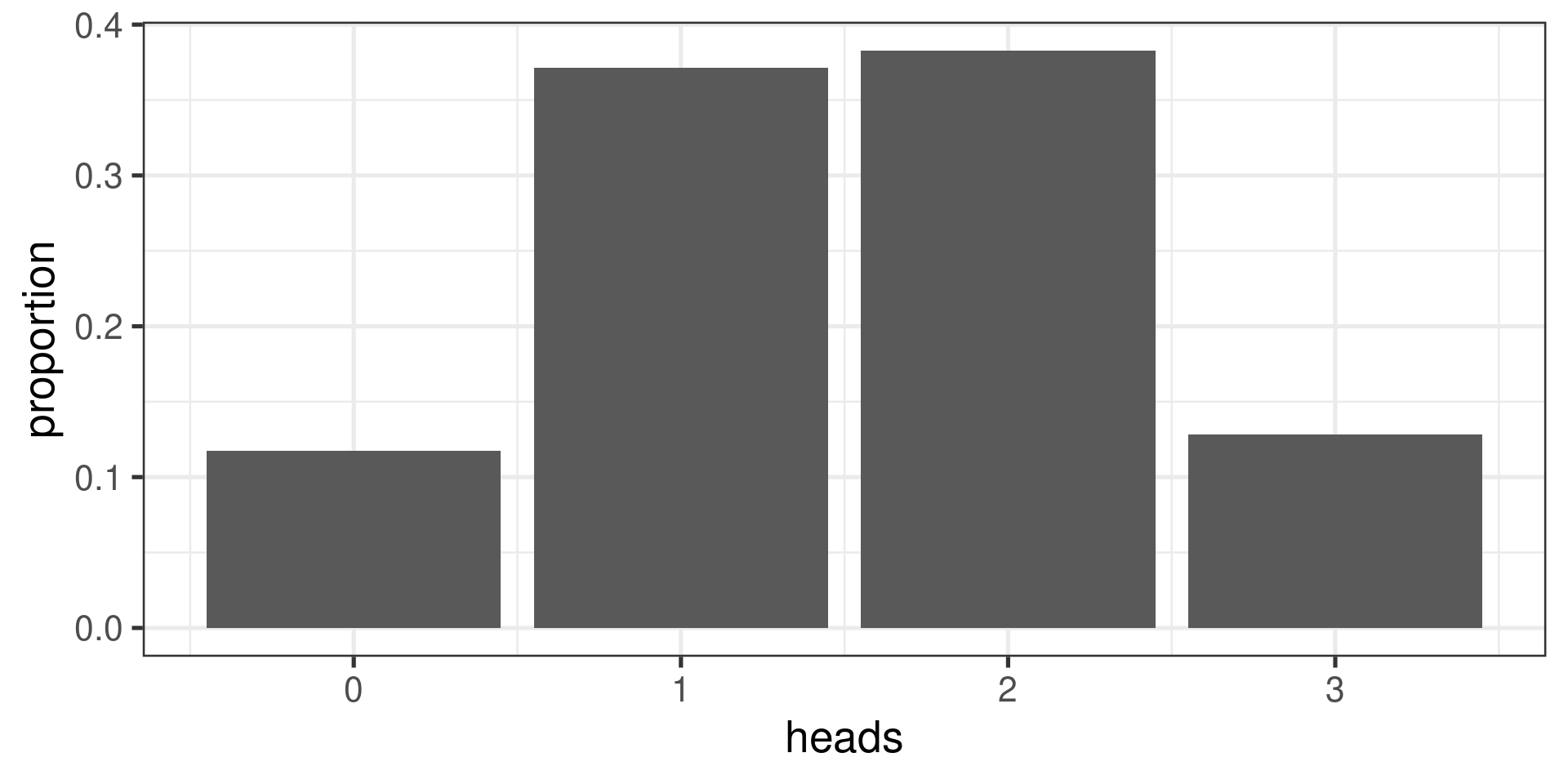
tosses <- do (10000) * rflip(3)
gf_props(~heads, data=tosses)Math 132B
Class 11
Summary of Probability Rules
- Addition rule for disjoint events: \(\operatorname{P}(A \text{ or } B) = \operatorname{P}(A) + \operatorname{P}(B)\)
- General addition rule: \(\operatorname{P}(A \text{ or } B) = \operatorname{P}(A) + \operatorname{P}(B) - \operatorname{P}(A \text{ and } B)\)
- Complementary events rule: \(\operatorname{P}(A^C) = 1 - \operatorname{P}(A)\)
- Multiplication rule for independent events: \(\operatorname{P}(A \text{ and } B) = \operatorname{P}(A)\cdot\operatorname{P}(B)\)
- General multiplication rule: \(\operatorname{P}(A \text{ and } B) = \operatorname{P}(A)\cdot \operatorname{P}(B \mid A)\)
Couple of experiments one more time
-
I flip a coin. If it lands heads up, I roll a regular die. If it lands tails up, I roll a die with three 2s and there 6s.
Find \(P(T \text{ and } 6)\)
-
I remove two tokens from a bag that contains 3 blue and 2 yellow tokens.
Find \(P(\text{both tokens are yellow})\)
Definition of a Random Variable
A random variable is a mathematical model of a random quantity (measurement, count)
It is a function that assigns each outcome from a sample space a number.
Example: The number of dots on the side of a die that is facing up.
Example: The total number of dots on the sides of two dice that are facing up.
Example: The number of infants that choose the friendly character.
Example: The height of a plant randomly selected from a field.
Example
\(X = {}\) the number of heads when flipping 3 coins:
Example
\(X\) models “the number of heads in 3 tosses of a fair coin”.
- \(X\) can take on the values 0, 1, 2, 3.
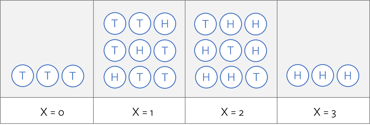
3 coin tosses
More examples:
Taking a token 3 times from a bag with one red and one blue token, with replacement. Counting the number of red tokens.
Asking 3 people to randomly select one of two characters, when they have no preference. Counting the number of times the friendly character was selected.
Randomly selecting 3 people from a large crowd that has 50% males and 50% females. Counting the number of females.
Randomly selecting 3 plants from a field in which 50% of the plants have some specific genetic mutation. Counting the number of plants with the mutation.
Mathematically, all of those are the same.
Distribution of a Random Variable
The distribution of a discrete random variable is the collection of its values and the probabilities associated with those values.
The probability distribution for \(X\) is as follows:
| \(x_i\) | 0 | 1 | 2 | 3 |
|---|---|---|---|---|
| \(P(X = x_i)\) | 1/8 | 3/8 | 3/8 | 1/8 |
The probabilities must add up to 1
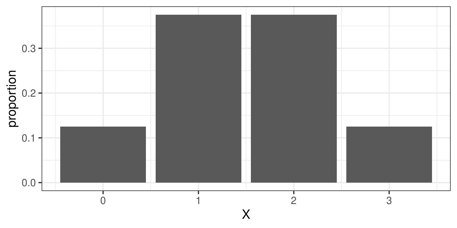
Bar graph showing a distribution
| \(x_i\) | 0 | 1 | 2 | 3 |
|---|---|---|---|---|
| \(P(X = x_i)\) | 1/8 | 3/8 | 3/8 | 1/8 |
Using a simulation to approximate a probability distribution
Expectation of a Random Variable
If \(X\) has outcomes \(x_1\), …, \(x_k\) with probabilities \(P(X=x_1)\), …, \(P(X=x_k)\), the expected value of \(X\), also called the mean of \(X\), is the sum of each outcome multiplied by its corresponding probability:
\[\begin{aligned} E(X) &= x_1 P(X=x_1) + x_2 P(X = x_2) + \cdots + x_k P(X=x_k)\\\\ &= \sum_{i=1}^{k}x_iP(X=x_i) \end{aligned}\]
The Greek letter \(\mu\) may be used in place of the notation \(E(X)\) and is sometimes written \(\mu_X\).
Expectation…
In the coin tossing example,
| \(x_i\) | 0 | 1 | 2 | 3 |
|---|---|---|---|---|
| \(P(X = x_i)\) | \(\color{red}1/8\) | \(\color{green}3/8\) | \(\color{blue}3/8\) | \(\color{orange}1/8\) |
\[\begin{align*} E(X) &= 0{\color{red}P(X=0)} + 1{\color{green}P(X=1)} + 2{\color{blue}P(X=2)} + 3{\color{orange}P(X = 3)} \\[1.2em] &\class{fragment}{{}= 0\cdot{\color{red}\frac{1}{8}} + 1\cdot{\color{green}\frac{3}{8}} + 2\cdot{\color{blue}\frac{3}{8}} + 3\cdot{\color{orange}\frac{1}{8}}} \\[1.2em] &\class{fragment}{{}= \frac{12}{8}} \\[1.2em] &\class{fragment}{{}= 1.5} \end{align*}\]
Expectation…
Intuitively, the expected value of \(X\) is approximately the number you would get if you took a lot of values of \(X\) and calculated the mean.
tosses <- do (10000) * rflip(3)
mean(~heads, data=tosses)
[1] 1.5054Variance and SD of a Random Variable
If \(X\) takes on outcomes \(x_1\), …, \(x_k\) with probabilities \(P(X=x_1)\), …, \(P(X=x_k)\) and has the expected value \(\mu=E(X)\), then the variance of \(X\), denoted by \(\operatorname{Var}(X)\) or \(\sigma^2\), is
\[\begin{align*} \operatorname{Var}(X) &= (x_1-\mu)^2 P(X=x_1) + (x_2 - \mu)^2 P(X = x_2) + \cdots+ (x_k-\mu)^2 P(X=x_k) \\ &= \sum_{j=1}^{k} (x_j - \mu)^2 P(X=x_j) \end{align*}\]
The standard deviation of \(X\), written as \(\operatorname{SD}(X)\) or \(\sigma\), is the square root of the variance. It is sometimes written \(\sigma_X\).
\[\operatorname{SD}(X) = \sqrt{\operatorname{Var(X)}}\]
Variance and SD…
In the coin tossing example,
| \(x_i\) | \(\color{red}0\) | \(\color{green}1\) | \(\color{blue}2\) | \(\color{orange}3\) |
|---|---|---|---|---|
| \(P(X = x_i)\) | \(\color{red}1/8\) | \(\color{green}3/8\) | \(\color{blue}3/8\) | \(\color{orange}1/8\) |
\[\begin{align*} \sigma_X^2 &= (x_1-\mu_X)^2P(X=x_1) + \cdots+ (x_4-\mu_X)^2 P(X=x_4) \\[1.2em] &= \left({\color{red}0} - \frac{3}{2}\right)^2{\color{red}\frac{1}{8}} + \left({\color{green}1} - \frac{3}{2}\right)^2{\color{green}\frac{3}{8}} + \left({\color{blue}2} -\frac{3}{2}\right)^2{\color{blue}\frac{3}{8}} + \left({\color{orange}3} -\frac{3}{2}\right)^2{\color{orange}\frac{1}{8}} \\[1.2em] &= \frac{3}{4} \end{align*}\]
The standard deviation \(\sigma_X\) is \(\sqrt{3/4} = \sqrt{3}/2 = 0.866\).
Standard Deviation …
Again, the standard deviation of \(X\) is approximately the number you would get if you took a lot of values of \(X\) and calculated the standard deviation of the data.
tosses <- do (10000) * rflip(3)
sd(~heads, data=tosses)
[1] 0.8713321Another example
Suppose your roll three fair six sided dice. Let \(X = \text{ the number of sixes rolled}\).
What are the possible values of \(X\)?
What is the probability distribution for \(X\)?
What is the expected value of \(X\)?
What is the variance of \(X\)?
Common theme
- Number of heads when tossing three fair coins
- Number of sixes when rolling three fair dice
- Number of heads when tossing 16 fair coins
- Number of infants choosing the helper, provided infants choose randomly.
All these can be modeled by so-called binomial random variables.
Binomial Random Variables
\(X\) is a binomial random variable if it represents the number of successes in \(n\) replications of an experiment where
- Each replicate is independent of the other replicates.
- Each replicate has two possible outcomes: either success or failure.
- The probability of success \(p\) in each replicate is constant.
This is also called a binomial process.
A binomial random variable takes on values \(0, 1, 2, \dots, n\).
The numbers \(n\) and \(p\) are called the parameters of the distribution.
We write \(X \sim \operatorname{Binom}(n, p)\).
The Binomial Distribution
Suppose \(X\sim \operatorname{Binom}(n,p)\). What is \(P(X = x)\)?
- \(n\) independent repetitions
- \(x\) successes, each with probability \(p\)
- \(n - x\) failures, each with probability \(1 - p\)
\[\begin{gather} P(\text{first } x \text{ are successes and last } n - x \text{ are failures}) = \\ \underbrace{p\cdot p\cdot p \cdots p}_{x\text{ times}}\cdot\underbrace{(1-p)\cdot(1-p)\cdots(1-p)}_{(n-x) \text{ times}} = p^x\cdot (1-p)^{n-x} \end{gather}\]
But also
\[\begin{gather} P(\text{first } n-x \text{ are failures and last } x \text{ are successes}) = \\ \underbrace{(1-p)\cdot(1-p)\cdots(1-p)}_{(n-x) \text{ times}} \cdot \underbrace{p\cdot p\cdot p \cdots p}_{x\text{ times}} = p^x\cdot (1-p)^{n-x} \end{gather}\]
or it may be that the first is success, then there are two failures, then a success, and so on.
How many different ways can we choose \(x\) successes out of \(n\) repetitions?
The Binomial Coefficient
The binomial coefficient \(\binom{n}{x}\) is the number of ways to choose \(x\) items from a set of size \(n\), where the order of the choices is ignored.
Mathematically,
\[\binom{n} {x} = \frac{\overbrace{n\cdot(n-1)\cdot(n-2)\cdots(n-x+1)}^{x \text{ factors}}} {\underbrace{x\cdot(x-1)\cdot(x-2)\cdots 1}_{x \text{ factors}}}\]
Examples
- Calculate \(\binom{7}{3}\)
- Calculate \(\binom{7}{6}\)
- Calculate \(\binom{10}{4}\)
- Calculate \(\binom{10}{6}\)
Formula for the binomial distribution
Let \(X\) = number of successes in \(n\) trials, and \(0 \le x \le n\).
\[P(X = x)=\binom{n}{x} p^x (1-p)^{n-x}\]
Parameters of the distribution:
\(n\) = number of trials
\(p\) = probability of success
Examples
-
Let \(n = 3\) and \(p = 1/2\).
Calculate \(P(X = 1)\).
-
Let \(n = 3\) and \(p = 1/6\).
Calculate \(P(X = 2)\).
-
Let \(n = 16\) and \(p = 1/2\).
Calculate \(P(X = 14)\).
(Hint: \(\binom{16}{14} = \binom{16}{2}\))
Mean and SD for a binomial random variable
For a binomial distribution with parameters \(n\) and \(p\), it can be shown that:
Mean = \(np\)
Standard Deviation = \(\sqrt{np(1-p)}\)
The derivation is not shown here nor in the text; it will not be asked for on a problem set or exam.
Binomial Probabilities in R
The function dbinom() is used to calculate \(P(X = k)\).
dbinom(k, size=n, prob=p): \(P(X = k)\)
For example, if \(X \sim \operatorname{Binom}(3, 1/6)\), the \(P(X = 2)\) is
dbinom(2, size=3, prob=1/6)[1] 0.06944444The d in dbinom stands for distribution or density.
Binomial Probabilities in R …
The function pbinom() is used to calculate \(P(X \leq k)\) or \(P(X > k)\).
-
\(P(X \leq k)\):
pbinom(k, size=n, prob=p) -
\(P(X > k)\):
pbinom(k, size=n, prob=p, lower.tail = FALSE)
The p stands for probability.
pbinom examples:
if \(X \sim \operatorname{Binom}(16, 1/2)\), then \(P(X \le 13)\) is
pbinom(13, size=16, prob=1/2)[1] 0.9979095while \(P(X \ge 14) = P(X > 13)\) is
pbinom(13, size=16, prob=1/2, lower.tail=FALSE)[1] 0.002090454or, equivalently:
1 - pbinom(13, size=16, prob=1/2)[1] 0.002090454