dbinom(2, size=3, prob=1/6)[1] 0.06944444Class 12
\(X\) is a binomial random variable if it represents the number of successes in \(n\) replications of an experiment where
\(X \sim \operatorname{Binom}(n, p)\).
Possible values: \(0, 1, 2, \dots, n\).
The binomial coefficient \(\binom{n}{x}\) is the number of ways to choose \(x\) items from a set of size \(n\), where the order of the choices is ignored.
Mathematically,
\[\binom{n} {x} = \frac{\overbrace{n\cdot(n-1)\cdot(n-2)\cdots(n-x+1)}^{x \text{ factors}}} {\underbrace{x\cdot(x-1)\cdot(x-2)\cdots 1}_{x \text{ factors}}}\]
Let \(X\) = number of successes in \(n\) trials, and \(0 \le x \le n\).
\[P(X = x)=\binom{n}{x} p^x (1-p)^{n-x}\]
Parameters of the distribution:
\(n\) = number of trials
\(p\) = probability of success
Let \(n = 3\) and \(p = 1/2\).
Calculate \(P(X = 1)\).
Let \(n = 3\) and \(p = 1/6\).
Calculate \(P(X = 2)\).
Let \(n = 16\) and \(p = 1/2\).
Calculate \(P(X = 14)\).
(Hint: \(\binom{16}{14} = \binom{16}{2}\))
For a binomial distribution with parameters \(n\) and \(p\), it can be shown that:
Mean = \(np\)
Standard Deviation = \(\sqrt{np(1-p)}\)
The derivation is not shown here nor in the text; it will not be asked for on a problem set or exam.
R
The function dbinom() is used to calculate \(P(X = k)\).
dbinom(k, size=n, prob=p): \(P(X = k)\)
For example, if \(X \sim \operatorname{Binom}(3, 1/6)\), the \(P(X = 2)\) is
dbinom(2, size=3, prob=1/6)[1] 0.06944444The d in dbinom stands for distribution or density.
R …The function pbinom() is used to calculate \(P(X \leq k)\) or \(P(X > k)\).
\(P(X \leq k)\):
pbinom(k, size=n, prob=p)
\(P(X > k)\):
pbinom(k, size=n, prob=p, lower.tail = FALSE)
The p stands for probability.
pbinom examples:if \(X \sim \operatorname{Binom}(16, 1/2)\), then \(P(X \le 13)\) is
pbinom(13, size=16, prob=1/2)[1] 0.9979095while \(P(X \ge 14) = P(X > 13)\) is
pbinom(13, size=16, prob=1/2, lower.tail=FALSE)[1] 0.002090454or, equivalently:
1 - pbinom(13, size=16, prob=1/2)[1] 0.002090454A discrete random variable takes on a finite number of values.
Number of heads in a set of coin tosses
Number of people who have had chicken pox in a random sample
A continuous random variable can take on any real value in an interval.
Height in a population
Blood pressure in a population
A general distinction to keep in mind: discrete random variables are counted, but continuous random variables are measured.
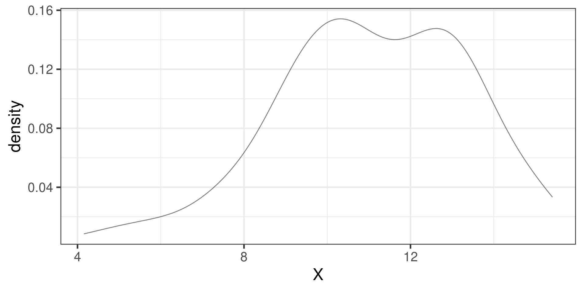
We use so-called density function or density curve.
The total area under the density curve is 1.
The probability that a variable has a value within a specified interval is the area under the curve over that interval.
When working with continuous random variables, probability is found for intervals of values rather than individual values.
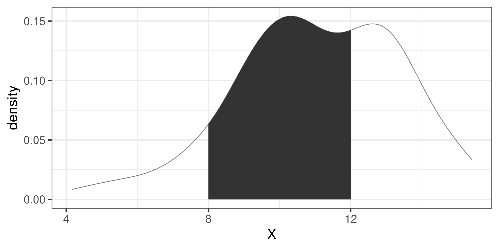
The probability that a continuous r.v. \(X\) takes on any single individual value is 0. That is, \(P(X = x) = 0\).
Thus, \(P(a < X < b)\) is equal to \(P(a \leq X \leq b)\).
The probability \(P(a \le X \le b)\) is given by the area under the density curve!
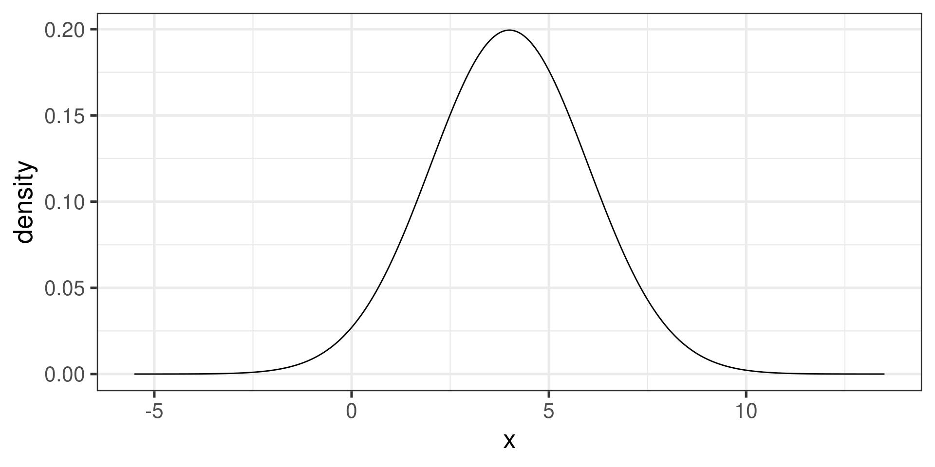
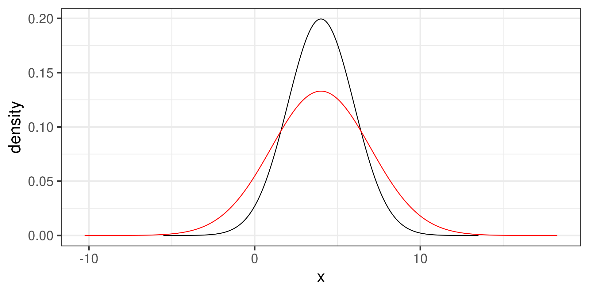
gf_dist("norm", params=c(mean = 4, sd = 2))gf_dist("norm", params=c(mean = 4, sd = 2)) |>
gf_dist("norm", mean = 4, sd = 3, color="red")Empirical Rule for normal distribution:
approximately 68% of the values are within 1 SD of the mean
approximately 95% of the values are within 2 SDs of the mean
approximately 99.7% of the values are within 3 SDs of the mean
68-95-99.7
The distribution of test scores on the SAT and the ACT are both nearly normal.
Suppose that one student scores an 1800 on the SAT (Student A) and another student scores a 24 on the ACT (Student B). Which student performed better?
The standard normal distribution is defined as a normal distribution with mean 0 and variance 1. It is often denoted as \(Z \sim N(0, 1)\).
Any normal random variable \(X\) can be transformed into a standard normal random variable \(Z\).
\[Z = \dfrac{X - \mu}{\sigma} \qquad X = \mu + Z\sigma\]
SAT scores are \(N(1500, 300)\). ACT scores are \(N(21,5)\).
\(x_A\) represents the score of Student A; \(x_B\) represents the score of Student B.
\[z_{A} = \frac{x_{A} - \mu_{SAT}}{\sigma_{SAT}} = \frac{1800-1500}{300} = 1 \]
\[z_{B} = \frac{x_{B} - \mu_{ACT}}{\sigma_{ACT}} = \frac{24 - 21}{5} = 0.6\]
What is the percentile rank for a student who scores an 1800 on the SAT for a year in which the scores are \(N(1500, 300)\)?
Calculate a \(Z\)-score. If \(X \sim N(\mu, \sigma)\), then \[Z = \frac{X - \mu}{\sigma},\] is a standard normal random variable, or, in symbols, \(Z \sim N(0,1)\).
(1800 - 1500)/300[1] 1Find the normal probability in one of the tables, or let R do the work:
pnorm(z) calculates the area (i.e., probability) to the left of \(z\)
pnorm(1)[1] 0.8413447R do all the work …What is the percentile rank for a student who scores an 1800 on the SAT for a year in which the scores are \(N(1500, 300)\)?
pnorm(1800, mean = 1500, sd = 300)[1] 0.8413447Which score on the SAT would put a student in the 99\(^{th}\) percentile?
Identify the \(Z\)-value from the table or using R: qnorm(p) calculates the value \(z\) such that for a standard normal variable \(Z\), \(p = P(Z \leq z)\).
qnorm(0.99) gives us 2.326348, or approximately 2.33.
Calculate the score, \(X\). If \(Z \sim N(0,1)\), then \[X = \sigma Z + \mu\] is Normal with mean \(\mu\) and standard deviation \(\sigma\), in symbols \(X \sim N(\mu, \sigma)\).
\[X = \sigma Z + \mu = 300(2.33) + 1500 = 2199\]
R do the work …Which score on the SAT would put a student in the 99\(^{th}\) percentile?
qnorm(0.99, mean = 1500, sd = 300)[1] 2197.904The q in qnorm stands for quantile.
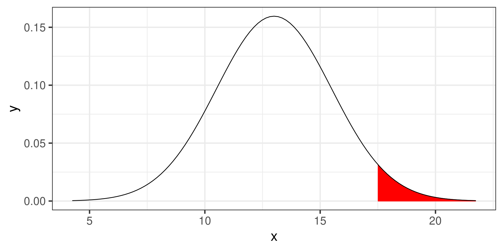
Find the probability that \(X \ge 17.5\) if \(X \sim N(13, 2.5)\)
Calculate the \(z\)-score:
\[z = \frac{17.5 - 13}{2.5} = 1.8\]
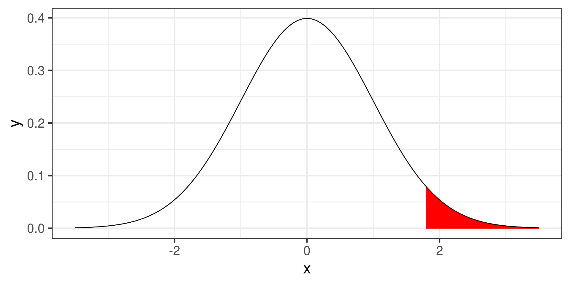
Now we need to find the area to the right of 1.8 under the standard normal curve.
Area to the right of 17.5.
Area to the right of 1.8.
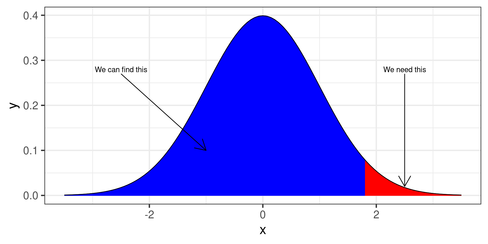
The total area under the normal curve is always 1.
All we need to do is subtract:
area to the right = 1 - area to the left
Finally, we can find the area to the right of 1.8.
1 - pnorm(1.8)[1] 0.03593032pnorm(1.8, lower.tail=FALSE)[1] 0.03593032