gf_dist("binom", params=c(size = 16, prob=1/2))Math 132B
Class 13
Binomial and Normal distributions
Binomial distributions have parameters \(n\) and \(p\): \(\operatorname{Binom}(n,p)\)
Normal distributions have parameters \(\mu\) and \(\sigma\): \(\operatorname{Norm}(\mu,\sigma)\)
Binomial distributions are discrete.
Normal distributions are continuous.
In both of them, we saw a similar “bell” shape.
The mean and standard deviation of a binomial distribution are \(\mu = np\) and \(\sigma = \sqrt{np(1-p)}\).
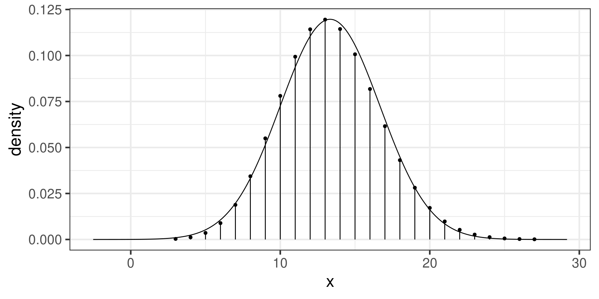
A binomial distribution
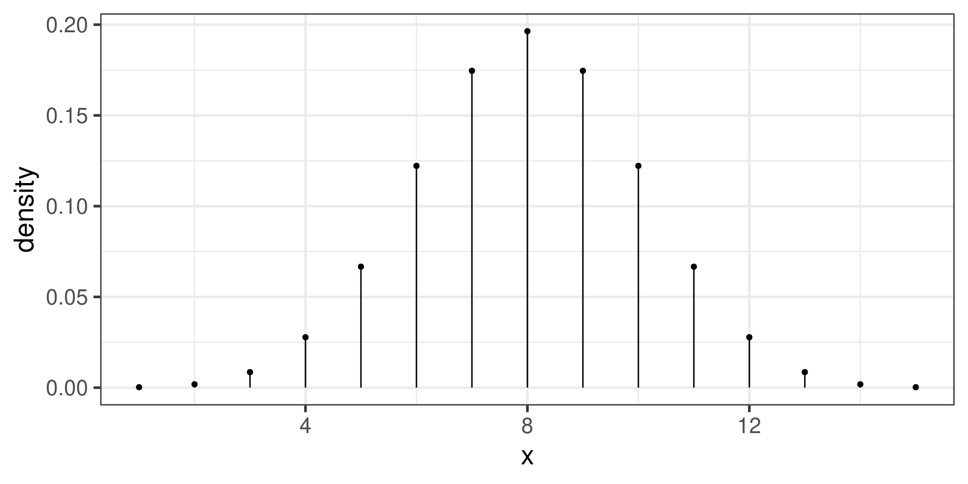
- Mean: \(\mu = n\cdot p = 16\cdot \frac{1}{2} = 8\)
- SD: \(\sigma = \sqrt{n\cdot p\cdot(1-p)} = \sqrt{4} = 2\)
Normal distribution \(\operatorname{Norm}(8, 2)\)
gf_dist("norm", params=c(mean=8, sd=2))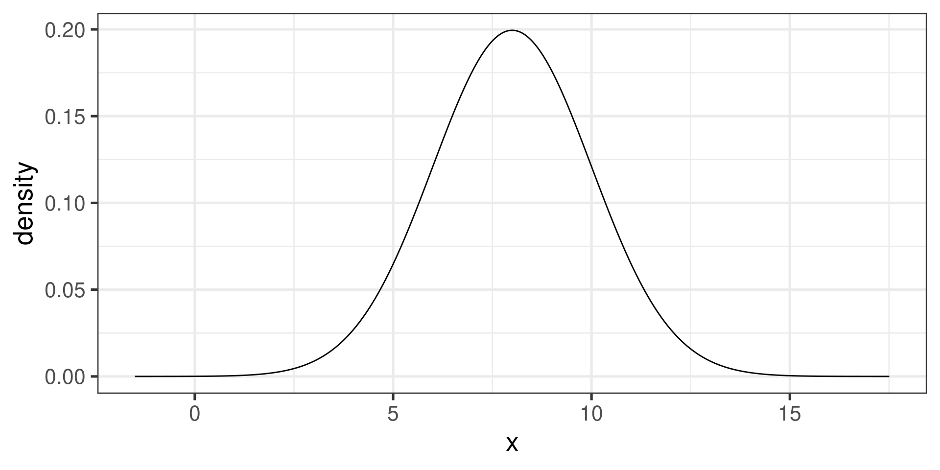
Normal and binomial distributions with the same \(\mu\) and \(\sigma\):
gf_dist("binom", params=c(size = 16, prob=1/2)) |>
gf_dist("norm", mean=8, sd=2, color="red")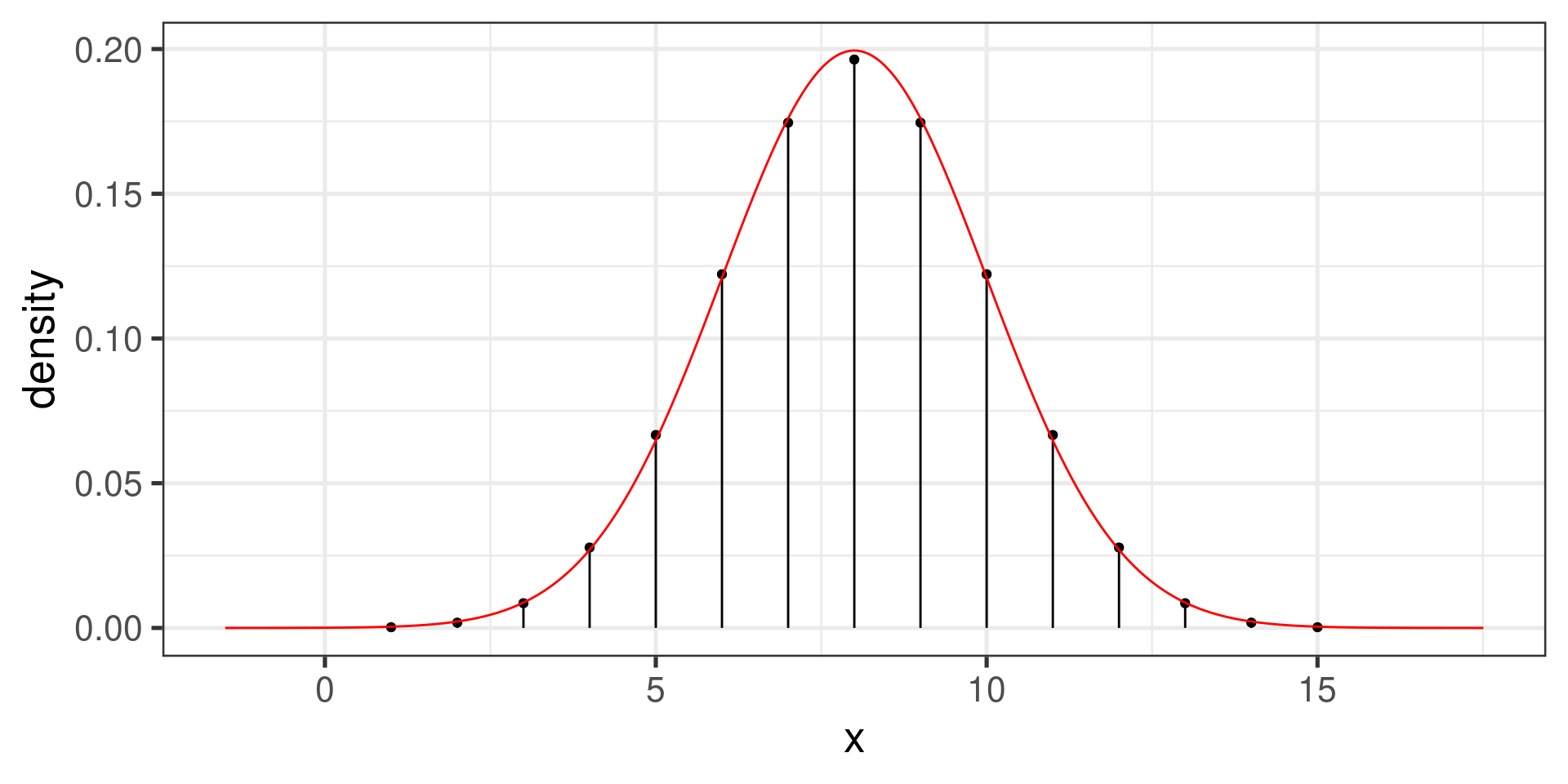
Simulation
flips <- do(10000) * rflip(16, prob=1/2)
gf_dhistogram(~heads, data = flips, binwidth=1, boundary=0.5) |>
gf_dist("norm", mean=8, sd=2, color="red")
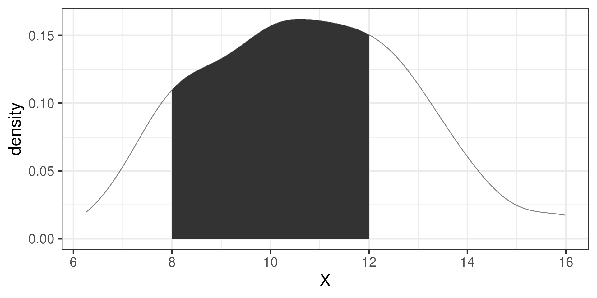
Density Histogram
We used gf_dhistogram instead of gf_histogram.
In density histogram, the area or each bar is the relative frequency of the corresponding bin.
The area of the whole density histogram is equal to 1.
That’s why we can compare it to a density curve of a random variable.
If \(X\sim\operatorname{Binom}(16, \frac{1}{2})\), what is \(\operatorname{P}(X \le 13)\)?
Compare
pbinom(13, size=16, prob=1/2)[1] 0.9979095to
pnorm(13.5, mean=8, sd=2)[1] 0.9970202Another example
Another example
Compare
pbinom(16, size=80, prob=1/6)[1] 0.8300908to
But
and
Compare
pbinom(1, size=12, prob=1/6)[1] 0.3813326to
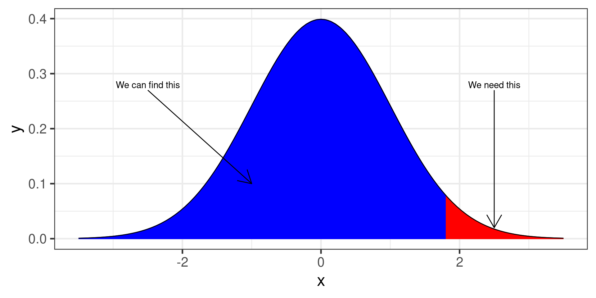
Approximating Binomial by Normal
If \(B\sim \operatorname{Binom}(n,p)\) and \(X \sim \operatorname{Norm}(\mu, \sigma)\) where \[\mu = np \text{ and } \sigma = \sqrt{np(1-p)},\]
sometimes we can approximate \(P(B \le k)\) by \(P(X \le k + 0.5)\)
or, similarly, \(P(B \ge k)\) by \(P(X \ge k - 0.5)\).
What’s sometimes: when \(np\) and \(n(1-p)\) are large enough!
Example
Suppose \(X\sim \operatorname{Binom}(100, 0.3)\)
Use the normal distribution to approximate \(\operatorname{P}(20 \le X \le 32)\).
Solution
Mean:
Standard deviation:
Interval:
z-scores:
Now we can use the normal probability tables
Few other useful distributions
“Counting” distributions:
Binomial: number of successes in \(n\) trials.
Poisson: number of occurrences in given time or space.
“Waiting time” distributions:
Geometric: how many trials until the first success.
Exponential: waiting time between two occurrences.
The Poisson distribution
The Poisson distribution is used to calculate probabilities for rare events that accumulate over time.
It used most often in settings where events happen at a rate \(\lambda\) per unit of population and per unit time, such as the annual incidence of a noninfectious disease in a population.
Typical example: for children ages 0 - 14, the incidence rate of acute lymphocytic leukemia (ALL) was approximately 30 diagnosed cases per million children per year in 2010.
Example: Outbreaks of childhood leukemia
Fortunately, childhood cancers are rare.
For children ages 0 - 14, the incidence rate of acute lymphocytic leukemia (ALL) was approximately 30 diagnosed cases per million children per year in the decade from 2000 - 2010. Approximately 20% of the US population are in this age range.
Some questions:
- What is the incidence rate over a 5 year period?
- In a small city of 75,000 people, what is the probability of observing exactly 8 cases of ALL over a 5 year period?
- In the small city, what is the probability of observing 8 or more cases over a 5 year period?
Poisson Distribution
Suppose events occur over time in such a way that
The probability an event occurs in an interval is proportional to the length of the interval.
Events occur independently at a rate \(\lambda\) per unit of time.
Then the probability of exactly \(x\) events occurring in one unit of time is \[ P(X = x) = \frac{e^{-\lambda}\lambda^{x}}{x!}, \,\, x = 0, 1, 2, \ldots \]
Notation: \(X \sim \operatorname{Pois}(\lambda)\)
Several units of time
The probability of exactly \(x\) events in \(t\) units of time is \[ P(X = x) = \frac{e^{-\lambda t}(\lambda t)^{x}}{x!}, \,\, x = 0, 1, 2, \ldots \] Notation: \(X \sim \operatorname{Pois}(\lambda t)\)
This is really just another Poisson distribution, with the rate multiplied by \(t\).
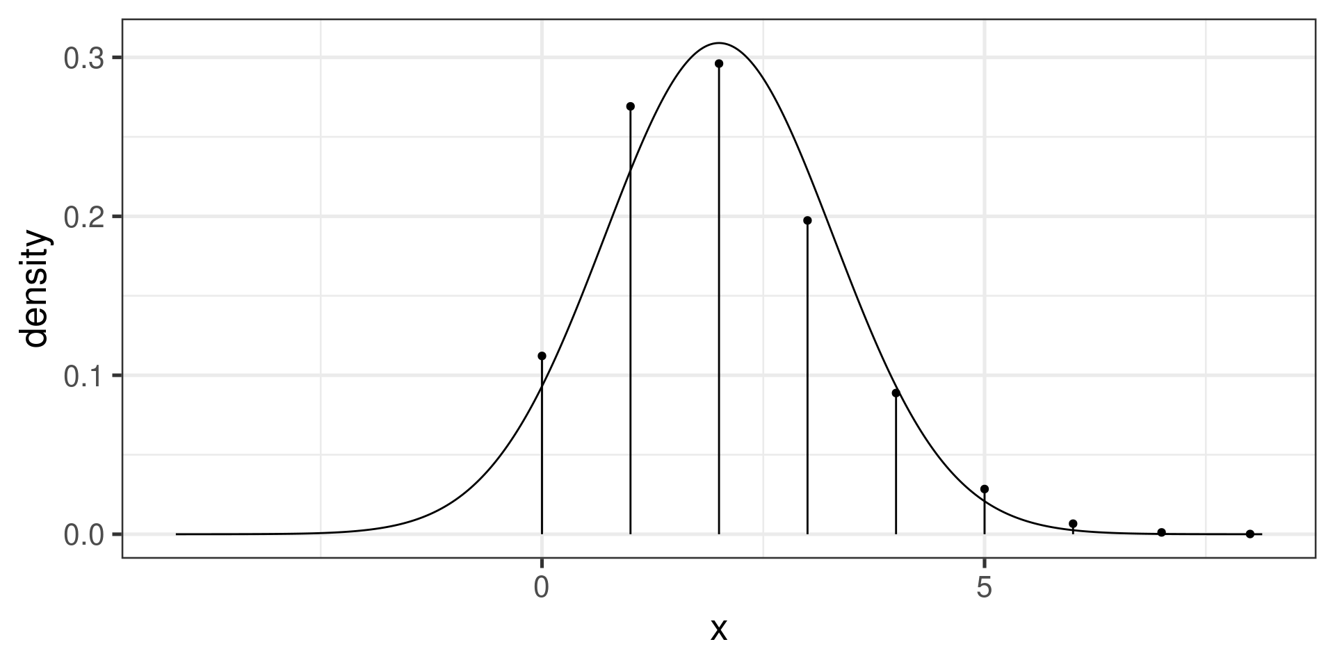
Example: Poisson distribution with \(\lambda = 2.25\)
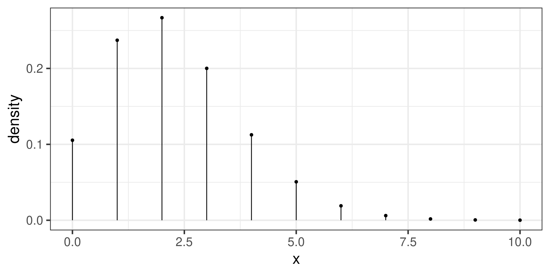
Poisson mean and standard deviation
For the Poisson distribution modeling the number of events that occur in one unit of time:
The mean is \(\lambda\).
The standard deviation is \(\sqrt{\lambda}\).
In \(t\) units of time, the mean and standard deviation are, respectively, \(\lambda t\) and \(\sqrt{\lambda t}\).
Childhood leukemia cases
(OI Biostat, Example 3.37)
The incidence rate of ALL in a year is 30 per 1,000,000 children:
- \(\dfrac{30}{1,000,000}= 0.00003 = 3\times 10^{-5}\).
The incidence rate over a 5-year period is \(5\cdot 30\) per 1,000,000 children:
- \(\dfrac{150}{1,000,000} = 0.00015 = 1.5 \times 10^{-4}\).
What about a city of size 75,000?
The incidence rate over a 5-year period is \(1.5\times 10^{-4}\).
About 20% of US population is in the range 0 - 14.
In a city of 75,000 people, approximately \((75,000)(0.20) = 15,000\) children will be age 0 - 14.
-
The five-year rate of new cases for the city would be:
\[(1.5 \times 10^{-4})(15,000) = 2.25\]
If \(X = {}\) the number of diagnosed cases of ALL in a city of size 75,000 over a 5-year period, then \[X \sim \operatorname{Pois}(2.25).\]
What is the probability of 8 cases over 5 years?
\[X \sim \operatorname{Pois}(2.25).\]
\[P(X=8) = \frac{e^{-\lambda}\lambda^{x}}{x!} = \frac{e^{(-2.25)}(2.25)^{8}}{8!}\]
Easiest to calculate this is in R.
Suppose \(X \sim \operatorname{Pois}(\lambda)\):
-
\(P(X = k)\) is
dpois(k, lambda = ...)so we need
dpois(8, lambda = 2.25)[1] 0.001717027
What is the probability of 8 or more cases?
Would 8 or more cases be a rare event?
- Calculate \(P(X \geq 8) = 1 - P(X \leq 7)\).
Suppose \(X \sim \operatorname{Pois}(\lambda)\):
-
\(P(X \le k)\) is
ppois(k, lambda = ...)1 - ppois(7, lambda = 2.25)[1] 0.002267088
Question
According to our model, the probability that a city of 75,000 will have 8 or more diagnosed cases of ALL over 5 years is about \(.2\)%.
Suppose that in certain city of that size, there are 8 cases diagnosed over 5 years, repeatedly.
What is going on?
Geometric Distribution
\(X\) is a geometric random variable if it represents the waiting time for the first success in a sequence of replications where
- Each replicate is independent of the other replicates.
- Each replicate has two possible outcomes: either success or failure.
- The probability of success \(p\) in each replicate is constant.
A geometric random variable takes on values \((0,) 1, 2, \dots\).
The only parameter is the probability of success \(p\).
We write \(X \sim \operatorname{Geom}(p)\).
Example
You repeatedly roll a fair die until you roll a ⚅.
\(X = {}\) the total number of rolls required.
Then \(X \sim \operatorname{Geom}(1/6)\).
What is the probability of getting the first ⚅ on the fourth roll: \(P(X = 4)\)?
\[P(X = 4) = \frac{5}{6}\cdot\frac{5}{6}\cdot\frac{5}{6}\cdot\frac{1}{6}\]
Different meaning of “waiting time”
You repeatedly roll a fair die until you roll a ⚅.
\(Y = {}\) the total number of failures before the first success.
We also say \(Y \sim \operatorname{Geom}(1/6)\).
What is the probability of getting the first ⚅ on the fourth roll: \(P(X = 4) = P(Y = 3)\)?
\[P(Y = 3) = \frac{5}{6}\cdot\frac{5}{6}\cdot\frac{5}{6}\cdot\frac{1}{6}\]
In R
R uses the second version: only failures are counted.
\(P(Y = 3)\):
dgeom(3, prob = 1/6)[1] 0.09645062\(P(Y \le 3)\):
pgeom(3, prob = 1/6)[1] 0.5177469Mean and standard deviation
-
For the \(X\) variable (the success is included in the count):
\[\mu = \frac{1}{p} \text{ and } \sigma = \sqrt{\frac{1-p}{p^2}}\]
-
For the \(Y\) variable (only counting the failures):
\[\mu = \frac{1-p}{p} \text{ and } \sigma = \sqrt{\frac{1-p}{p^2}}\]
Another example
Suppose we have a large population in which 2% of individuals have certain disease. We want to find one individual with the disease.
\(X=\) the total number of individuals we need to test.
\(Y=\) the number of healthy individuals we need to test before finding one with the disease.
We will say that \(Y \sim \operatorname{Geom}(0.02)\).
Question:
Why did we assume the population is large?
Distributions Summary Table
| Distribution: | Binomial | Normal | Poisson | Geometric |
|---|---|---|---|---|
| Parameters: | \(n\), \(p\) | \(\mu\), \(\sigma\) | \(\lambda\) | \(p\) |
| Possible values: | \(0,1,\ldots,n\) | (-\(\infty\), \(\infty\)) | \(0,1,\ldots\) | \(0,1,\ldots\) |
| Mean: | \(np\) | \(\mu\) | \(\lambda\) | \(\frac{1-p}{p}\) |
| Standard Dev.: | \(\sqrt{np(1-p)}\) | \(\sigma\) | \(\sqrt{\lambda}\) | \(\sqrt{\frac{1-p}{p^2}}\) |
| \(P(X = x)\): | dbinom(...) |
0 | dpois(...) |
dgeom(...) |
| \(P(X \le x)\): | pbinom(...) |
pnorm(...) |
ppois(...) |
pgeom(...) |