Math 132B

Class 16

What is statistical inference?

Goal: Create or evaluate a mathematical model for some random variable(s), using a sample of its (their) values.

Model for a random variable: A distribution with some parameters.

What can we learn from a sample?

Last time we set up an experiment:

We took all values of the height variable from the very large YRBSS data set. We used that as population.
We chose a sample size \(n\), and collected a large number (1000) samples of size \(n\) from the population.
We calculated the mean of each sample.
We looked at the distribution of these means.

What did we learn

The sample means varied from sample to sample.
There was less variation with larger samples!
The distribution of the sample means was kind of bell shaped.
More so with larger samples.
The mean of the sample means seemed to be the same as the mean of the population.
The standard deviation of the sample means was consistently equal to \[\frac{\sigma}{\sqrt{n}}\] where \(\sigma\) was the population standard deviation.

Some notation and terminology

We took a random variable \(X\): the height of a random person in the population.
We chose a sample size \(n\), collected a sample of size \(n\), and calculated the mean. We call this the sample mean.
We were asking if we can use this mean to estimate the population mean.
The calculated sample mean gives us a point estimate of the population mean.
Big question: How good is this estimate?
The difference between the sample mean and the population mean is called the sampling error.

Some more notation and terminology

We took a random variable \(X\): the height of a random person in the population.
We chose a sample size \(n\), collected a sample of size \(n\), and calculated the mean.
This gives us a new random variable, so-called sample mean: \[\overline{X} = \overline{X}_n = \text{ the mean of sample of size n drawn from } X.\]
The distribution of \(\overline{X}\) is called a sampling distribution for means.
Sampling error: \(\overline{X} - \text{ population mean}\).
The standard deviation of \(\overline{X}\) is called the standard error of sample means.

What did we learn, again

For large samples, the sampling distribution of sample means is close to Normal.
The mean of the sampling distribution is the same as the mean of the population \(\mu\).
The standard error of sample means depends of the standard deviation of the population and on the sample size: \[SE\left(\overline{X}_n\right) = \frac{\sigma}{\sqrt{n}}.\]
We can model the sampling distribution as \[N\left(\mu, \frac{\sigma}{\sqrt{n}}\right)\]
This is known as the Central Limit Theorem for sample means.

Use a sample to find an estimate for one parameter of the model.

Requires no previous knowledge of the parameter, although we may have to make some assumptions about the model.

We have a model that we think may work, and we want to test it against our data.

We want to see whether the model is consistent with the data.

Point estimates

Suppose I use the sample mean to estimate the population mean.

We know that most of the time the estimate will be pretty good.

What does most of the time mean?
What does pretty good mean?

Confidence intervals

A confidence interval provides an estimate for a population parameter along with a margin of error that gives a plausible range of values for the population parameter.

A confidence interval for a population mean \(\mu\) has the general form \[\overline{x} \pm m \text{, or } (\overline{x} - m, \overline{x} + m), \] where \(m\) is the margin of error.

To calculate \(m\), we use what is known about the sampling distribution of \(\overline{X}\).

\[\overline{X} \sim N\left(\mu, \frac{\sigma}{\sqrt{n}}\right)\]

Unfortunately, we usually do not know \(\sigma\)!

Some useful notation

\(\mu\): unknown population mean
\(\sigma\): unknown population standard deviation
\(n\): the number of observations in a sample drawn from the population
\(\overline{x}\): sample mean from a sample taken from the population
\(s\): calculated sample standard deviation from the same sample used to calculate \(\overline{x}\)

An Idea

Instead of using \(\sigma\), use \(s\) (the sample standard deviation)!
Unfortunately, that will introduce an extra error, especially for small samples.
We will not be able to use a normal distribution.

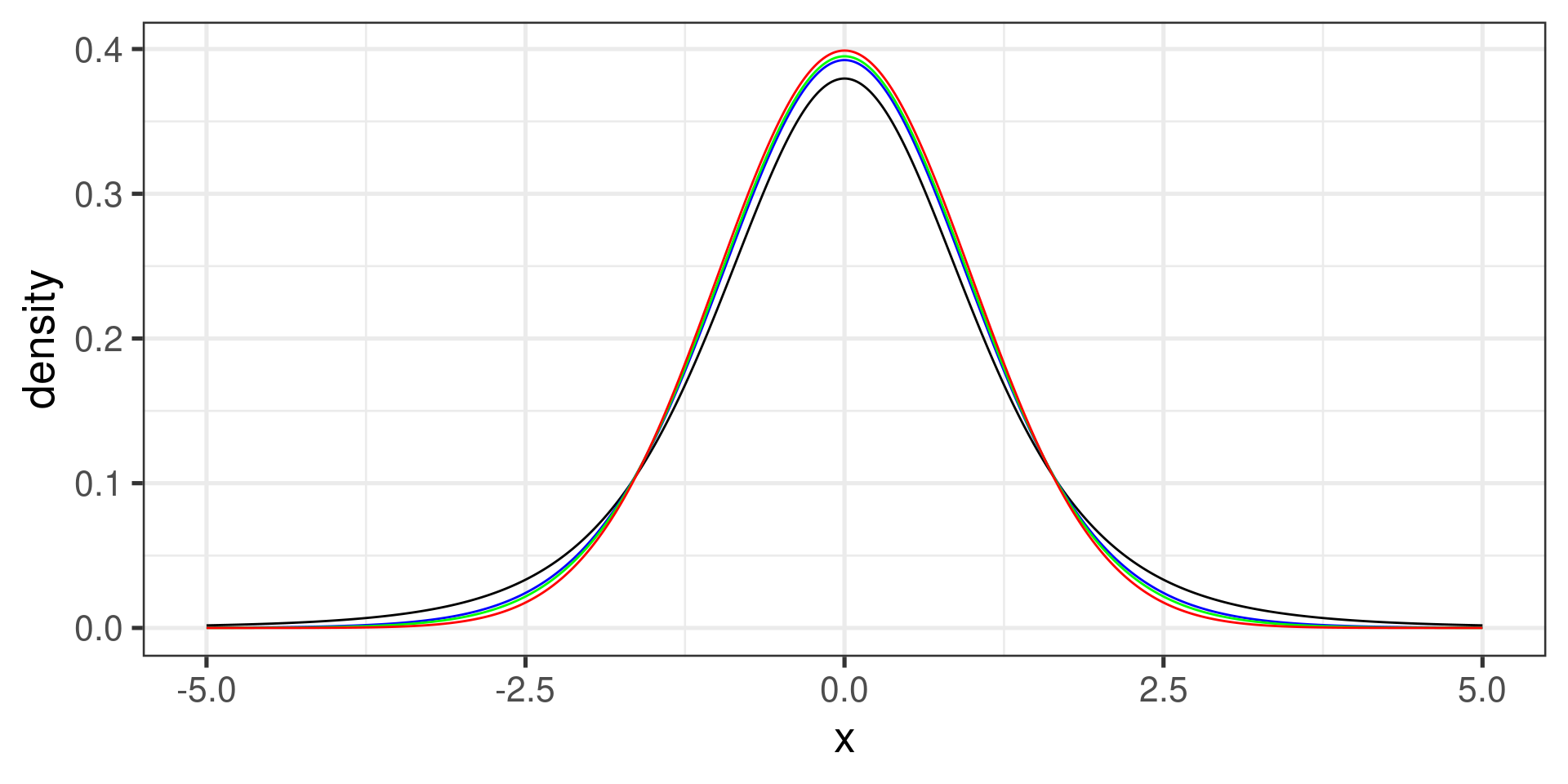
The \(t\) Distribution

The \(t\) distribution is symmetric, bell-shaped, and centered at 0.

It is very close to the standard normal distribution, but has one additional parameter called degrees of freedom (df).

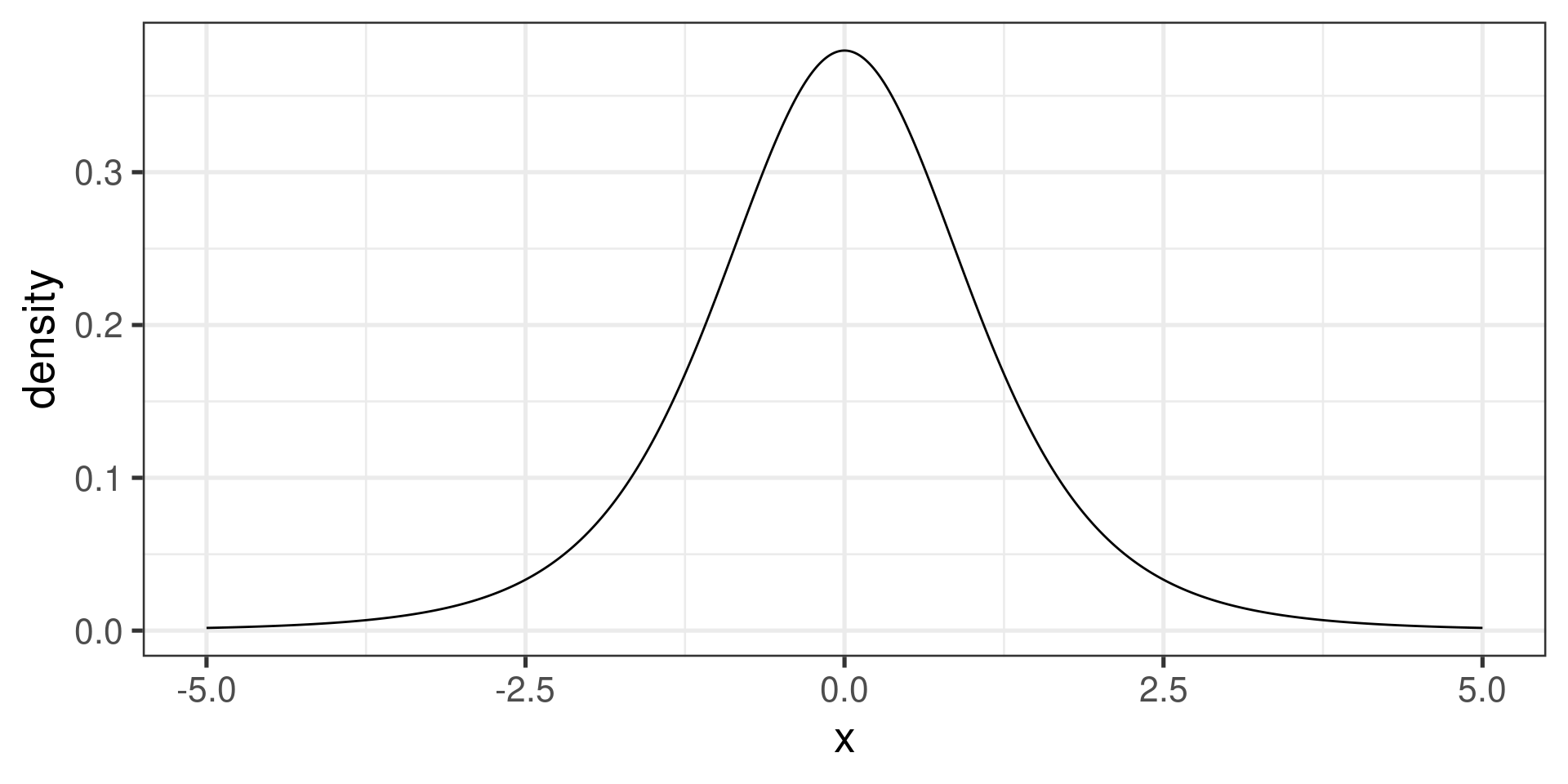
The tails of a \(t\) distribution are thicker than those in a normal distribution. This adjusts for the variability introduced by using \(s\) as an estimate of \(\sigma\).
When \(df\) is large (\(df \geq 30\)), the \(t\) and \(z\) distributions are virtually identical.

The \(t\) Distribution…

Important Discovery

In 1908, W. S. Gosset (a.k.a. “Student”) discovered that if the population is normally distributed then the quantity

\[t = \frac{\overline{X} - \mu}{\frac{s}{\sqrt{n}}}\]

has a \(t\) distribution with \(n-1\) degrees of freedom.

The standard error for \(\overline{X}\)

Central Limit Theorem:

The standard deviation of the random variable \(\overline{X}\) is

\[\text{SD}_{\overline{X}} = \dfrac{\sigma_x}{\sqrt{n}}\]

Thus, the variability of a sample mean is inversely proportional to the square root of the sample size.

Typically, \(\sigma_x\) is unknown and estimated by \(s_x\).
The term \(\frac{s_x}{\sqrt{n}}\) is what we usually mean by standard error of \(\overline{X}\).

General Form for a Confidence Interval

A \(100\cdot(1 - \alpha)\)% confidence interval for \(\mu\) is given by \[\overline{x} \pm t^\star \times \dfrac{s}{\sqrt{n}} = \left(\overline{x} - t^\star \times \dfrac{s}{\sqrt{n}}, \overline{x} + t^\star \times \dfrac{s}{\sqrt{n}}\right)\] where \(t^\star\), the critical \(t\)-value, is the point on a \(t\) distribution with \(n-1\) degrees of freedom that has area:

\(1 - \alpha/2\) to the left and
\(\alpha/2\) to the right.

The quantity \(100\cdot(1 - \alpha)\)% is called confidence level and denoted by \(L\).

The critical \(t\)-value

The ‘confidence level’

The confidence level is also called the confidence coefficient.

The correct interpretation:

The method illustrated for computing a 95% confidence interval will produce an interval that (on average) contains the true population mean 95 times out of 100.
5 out of 100 will be incorrect,
unfortunately, we do not know whether a particular interval contains the population mean.

Confidence Intervals

jstat = require("jstat")

viewof conf_level = Inputs.range(
  [50, 99], 
  {value: 95, step: 1, label: "CL (%):"}
)

viewof sample_size = Inputs.range(
  [5, 100], 
    {value: 25, step: 1, label: "n:"}
)

viewof resample = Inputs.button(
"Resample"
)

intervals = {
resample;
var gen_interval = function(i, size, L){
    var sample = Array.from({length: size}, function(){ return jstat.jStat.normal.sample(0,1)});
    var crit = jstat.jStat.studentt.inv(1 - (1 - L/100)/2, size-1);
    var xbar = jstat.jStat.mean(sample);
    var sd = jstat.jStat.stdev(sample);
    var merror = crit*sd/Math.sqrt(size);
    return {int: i + 1, low: xbar - merror, high: xbar + merror, fail: Math.abs(xbar) >= merror};
}
return Array.from({length: 100}, (_, i) => gen_interval(i, sample_size, conf_level));
}

Plot.plot({
width: 1000,
x: {ticks: false},
y: {domain: [-3, 3], grid: false},
color: {scheme: "BuRd"},
marks: [
Plot.ruleY([0]),
Plot.ruleX(intervals, {x: 'int', y1: 'low', y2: 'high', stroke: 'fail',
strokeWidth: 4})]
})

failed = d3.sum(intervals, i => i.fail)
ivaltxt = failed == 1? "1 failed interval" : failed + " failed intervals"

100 samples from the standard normal distribution, .

Accuracy vs. Precision

Accuracy is given by the confidence level. This tells you how likely you are to “hit the target”.
Precision is determined by the margin of error. This tells you how precisely is the target determined when you hit it.
If you want to increase the accuracy, you have to decrease the precision, and vice versa.
You can increase one without sacrificing the other by increasing the sample size.

Important assumptions

The data used to calculate the confidence interval are from a simple random sample taken from the target population.
One of the following has to be true:
1. The population is normally distributed with (unknown) mean \(\mu\) and (unknown) standard deviation \(\sigma\).
2. The sample size is at least 30, and the population is not visibly skewed.
3. If the population is skewed, larger sample is needed (several hundreds).

Two-sided Confidence Interval

A \(100\cdot(1 - \alpha)\)% CI for \(\mu\) is given by \[\overline{x} \pm t^\star \times \dfrac{s}{\sqrt{n}} = \left(\overline{x} - t^\star \times \dfrac{s}{\sqrt{n}}, \overline{x} + t^\star \times \dfrac{s}{\sqrt{n}}\right) \] where \(t^\star\), the critical \(t\)-value, is the point on a \(t\) distribution with \(n-1\) degrees of freedom that has area \((1 - \alpha/2)\) to the left (and area \(\alpha/2\) to the right).

One-sided confidence intervals (left)

A left or lower \(100\cdot(1 - \alpha)\)% CI for \(\mu\) is given by \[\left(\overline{x} + t^\star \times \dfrac{s}{\sqrt{n}}, \infty\right) \] where \(t^\star\), the critical \(t\)-value, is the point on a \(t\) distribution with \(n-1\) degrees of freedom that has area \(\alpha\) to the left (and area \(1 - \alpha\) to the right).

One-sided confidence intervals (right)

A right or upper \(100\cdot(1 - \alpha)\)% CI for \(\mu\) is given by \[\left(-\infty, \overline{x} + t^\star \times \dfrac{s}{\sqrt{n}}\right),\] where \(t^\star\), the critical \(t\)-value, is the point on a \(t\) distribution with \(n-1\) degrees of freedom that has area \(\alpha\) to the right (and area \(1 - \alpha\) to the left).