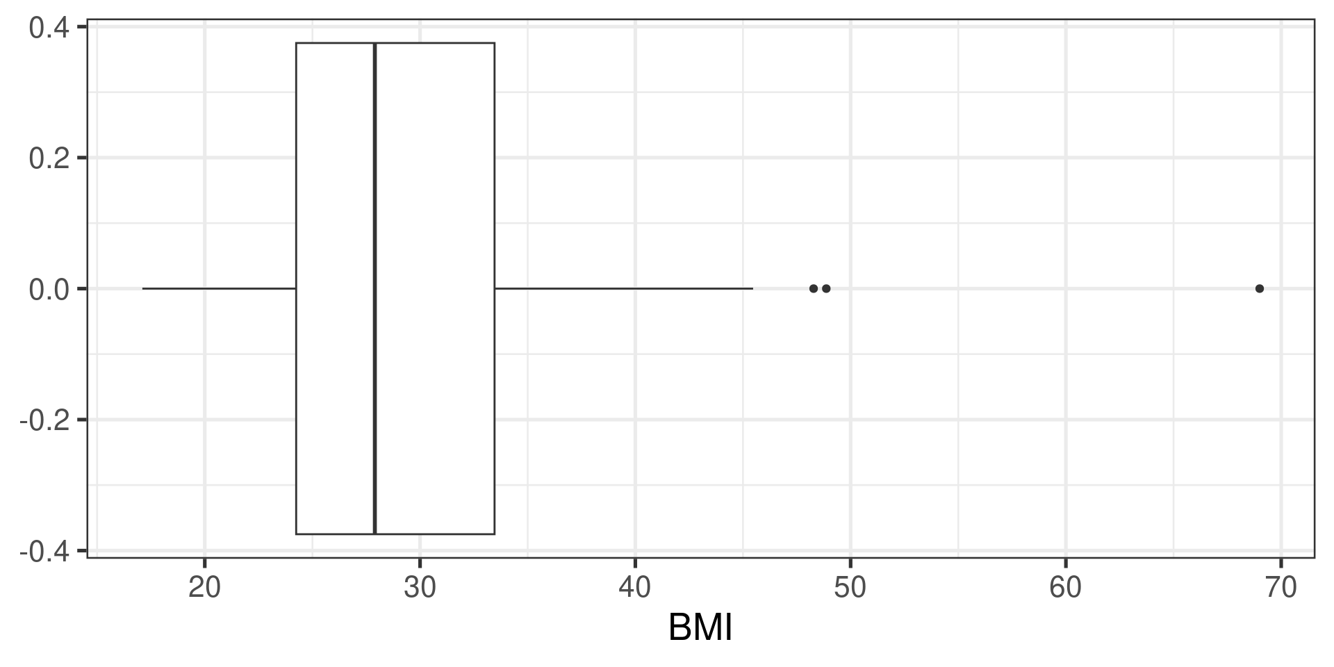
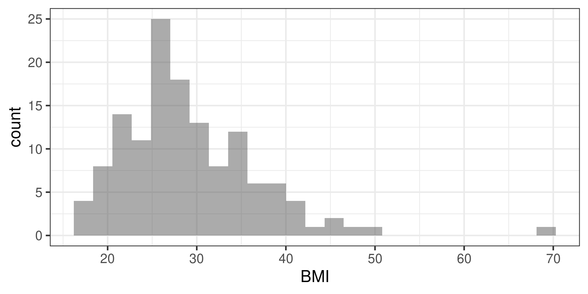
  min     Q1 median    Q3 max     mean       sd   n missing
17.1 24.245 27.9 33.46 69 29.09956 7.552866 135 0Math 132B
Class 17
Falsifying mathematical models
Do Americans tend to be overweight?
Body mass index (BMI) is an approximate scale used to assess weight status that adjusts for height.
When weight is measured in kg and height in meters, \[\text{BMI} = \frac{\text{weight}}{\text{height}{^2}}\]
When weight is measured in lbs and height in inches, \[\text{BMI} = \left(\frac{\text{weight}}{\text{height}{^2}}\right)(703)\]
WHO standards for BMI
| Category | BMI range |
|---|---|
| Underweight | \(<18.50\) |
| Normal (healthy weight) | 18.5-24.99 |
| Overweight | \(\geq 25\) |
| Obese | \(\geq30\) |
The National Health and Nutrition Survey (NHANES)
The National Health and Nutrition Examination Survey (NHANES) is another survey conducted by the CDC.
Purpose: to assess the health and nutritional status of adults and children in the United States
The
NHANESdataset in theNHANESpackage contains responses from 10,000 participants.The
nhanes.samp.adultdataset in theoibiostatpackage contains responses from a random sample from participants who were age 21 or older.
We will treat nhanes.samp.adult as our sample and think of the adult participants in the NHANES dataset as the population.
The NHANES sample
The NHANES sample…
Two approaches to the problem
I. Calculate a confidence interval for the population mean BMI.
- Use the formal logic of hypothesis testing.
I. Calculating a 95% confidence interval
- Calculate sample mean \(\bar{x}\)
- Calculate sample standard deviation \(s\).
- Figure out the sample size \(n\).
- Plug into the formula.
  min     Q1 median    Q3 max     mean       sd   n missing
 17.1 24.245   27.9 33.46  69 29.09956 7.552866 135       0
I. Calculating a 95% confidence interval
- \(\bar{x} = 29.0995556\)
- \(s = 7.5528657\)
- \(n = 135\)
- \(df = n - 1 = 134\)
\[SE = \frac{s}{\sqrt{n}}\]
Critical t
I. Calculating a 95% confidence interval
\(\bar{x} = 29.0995556\)
\(SE = 0.6500472\)
-
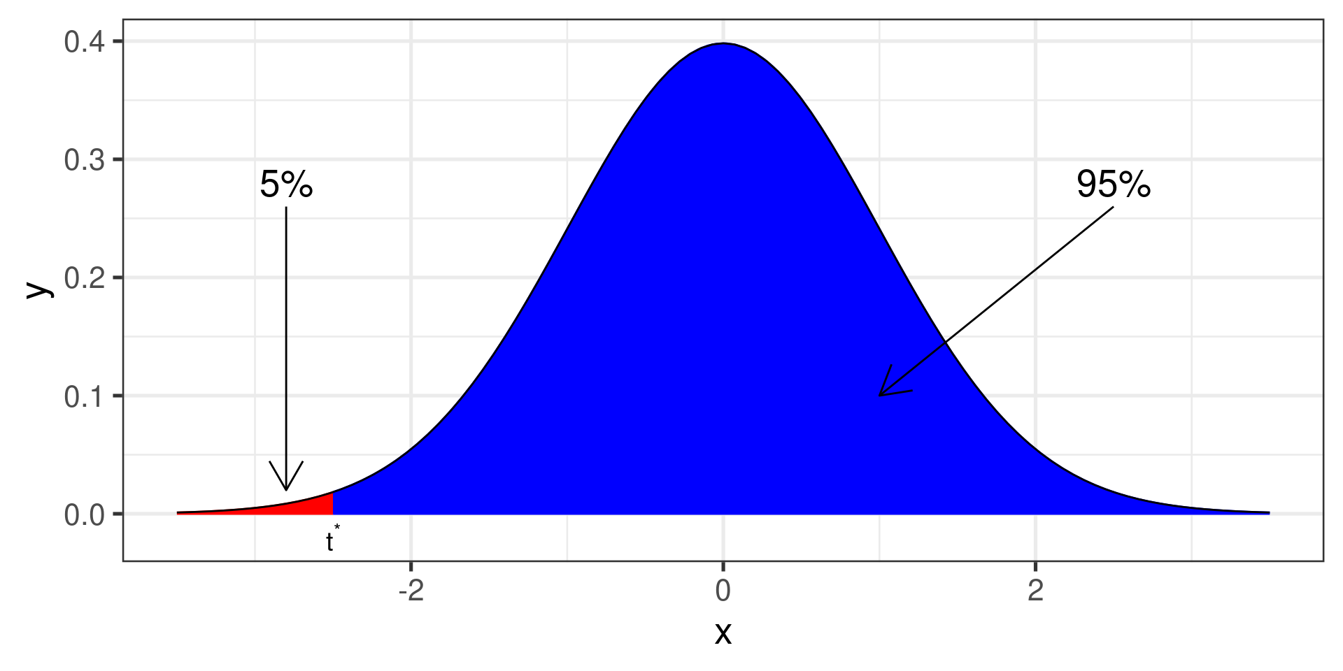
Critical \(t\):
qt(.05, df = 134)[1] -1.656305
Interval: \(\left(\bar{x} + t^*\cdot SE, \infty\right)\)
Confidence interval suggests that population average BMI is well outside the range defined as normal, 18.5 - 24.99.
Finding critical \(t\)-score :
We need \(\alpha = 1 - L\) and \(n\) for degrees of freedom. \(df = n - 1\)
-
Left or lower CI: the area to the left of \(t^\star\) is \(\alpha\).
With \(\alpha = 0.05\) (\(95\)% CI) and \(n = 25\):
qt(0.05, df = 24)[1] -1.710882 -
Right or upper CI: the area to the left of \(t^\star\) is \(1 - \alpha\).
With \(\alpha = 0.05\) (\(95\)% CI) and \(n = 25\):
qt(0.95, df = 24)[1] 1.710882 -
Two-sided CI: the area to the left of \(t^\star\) is \(1 - \alpha/2\).
With \(\alpha = 0.05\) (\(95\)% CI) and \(n = 25\):
qt(0.975, df = 24)[1] 2.063899
Using a table

Make the \(t^\star\) negative for left (lower) interval.
II. Formal approach to hypothesis testing
We have a mathematical model for the population.
Using this model, we calculate the probability of observing the sample statistic that was actually observed.
If this probability is extremely low, we conclude that there is something wrong with the model.
We have done this before!
-
The Infant Cognition Study
Model: the infants choose randomly (\(\operatorname{Binom}(16, 1/2)\)).
Observation: 14 out of 15 infants chose the helper.
\(\operatorname{P}(\text{Observation}\mid\text{Model}) \approx 0.002\)
-
The ALL example
Model: \(\operatorname{Pois}(2.25)\)
Observation: 8 cases of ALL over 5 years period.
\(\operatorname{P}(\text{Observation}\mid\text{Model}) \approx 0.002\)
Formal approach (OI Biostat Section 4.3.1)
Steps in hypothesis testing. Details coming in subsequent slides.
Formulate null and alternative hypotheses
Specify a significance level, \(\alpha\)
Calculate a test statistic
Calculate a \(p\)-value
State a conclusion in the context of the original problem
1. Null and alternative hypotheses
The null hypothesis (\(H_0\)) represents our mathematical model that we are trying to falsify.
The alternative hypothesis (\(H_A\)) claims a ‘real’ difference between the distribution of the observed data and the null-hypothesized distribution.
That is, the discrepancy between \(\overline{x}\) and \(\mu\) is large enough that it seems unlikely to occur from sampling variability.
1. Null and alternative…
Several possible choices for \(H_0\) and \(H_A\) for our BMI question. Let’s choose
\(H_0: \mu_{\text{bmi}} = 24.99 = \mu_0\)
\(H_A: \mu_{\text{bmi}} > 24.99\)
2. Specifying a significance level \(\alpha\)
Deciding what will “extremely small” mean.
The significance level \(\alpha\) can be thought of as the value that quantifies how rare or unlikely an event must be in order to represent sufficient evidence against \(H_0\).
Typically, \(\alpha\) is chosen to be \(0.05\), \(0.01\), or some other small value.
In the context of decision errors, \(\alpha\) is the probability of making a Type I error.
Type I error refers to incorrectly rejecting the null hypothesis.
More on this later.
Choose \(\alpha = 0.05\).
3. Calculate a test statistic
The test statistic measures the discrepancy between the observed data and what would be expected if the null hypothesis were true.
- Specifically, how many standard deviations is the observed sample value from the population value under the null hypothesis?
When testing hypotheses about a mean, the test statistic is
\[T = \frac{\overline{X} - \mu_0}{s/\sqrt{n}},\]
where the test statistic \(T\) follows a \(t\) distribution with \(n-1\) degrees of freedom.
In our example
- \(\bar{x} = 29.0995556\)
- \(s = 7.5528657\)
- \(n = 135\)
- \(H_0: \mu = 24.99\)
\[t = \frac{\bar{x} - \mu_0}{s/\sqrt{n}}\]
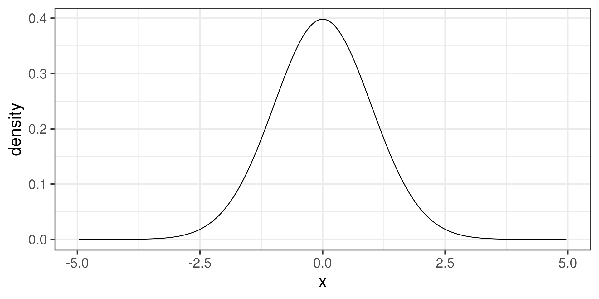
4. Calculate a \(p\)-value
Assuming our model is correct, the \(T\)-statistic has T distribution with \(n-1\) degrees of freedom.
In that case, what is the probability that T = 6.3219343?
What is the probability that we would observe a result equal to or more extreme than the observed sample value, if the null hypothesis is true?
- This probability is called the \(p\)-value.
- The \(p\)-value is not the probability that \(H_0\) is true!
- The \(p\)-value is not the probability that \(H_A\) is false!
- A result is considered unusual under the null model if its \(p\)-value is less than \(\alpha\).
4. The \(p\)-value…
For a right-sided alternative, \(\mu > \mu_0\), the \(p\)-value is the total area in the right tail of the t distribution that are beyond the value of the observed statistic.
4. The \(p\)-value…
The \(p\)-value measures how well does the null model explain the data.
The smaller the \(p\)-value, the stronger the evidence against the null model.
If the \(p\)-value is as small or smaller than \(\alpha\), we reject the null model as not being useful. We say that the result is statistically significant at level \(\alpha\). That means we falsified our mathematical model.
If the \(p\)-value is larger than \(\alpha\), we do not reject the null model. The result is not statistically significant at level \(\alpha\). In other words, the evidence does not contradict the null hypothesis.
What does small \(p\)-value really mean?
The \(p\) value is the conditional probability of a simple random sample of size \(n\) having the \(t\)-statistic equal to or more extreme than the sample we have, given the null model is correct.
Small \(p\)-value could mean:
We have a really strange sample (unlikely if sample is simple random, but quite possible if it is not!)
-
There is something wrong with the model:
- Maybe we used a wrong distribution? (Assumptions not satisfied)
- Maybe the null hypothesis is false.
Typical Conclusion
If the \(p\)-value is smaller than the significance level \(\alpha\), we reject the null hypothesis \(H_0\).
If the \(p\)-value is larger than \(\alpha\), we do not reject \(H_0\).
A subtle but important point: not rejecting \(H_0\) is not the same as proving that \(H_0\) is true. We simply do not have sufficient evidence that \(H_0\) is not true!
What it means is that the null model is reasonable enough, and we can keep using it.
Remember: all models are wrong!
In our example
\(H_A: \mu > 24.99\), so more extreme means larger (right tailed test).
- \(t = 6.3219343\)
- \(df = n - 1 = 134\)
1 - pt(6.32, df = 134)[1] 1.797873e-09The \(p\)-value is about \(0.000,\!000,\!001,\!78\), way smaller than \(\alpha\).
Finding the \(p\)-value
Suppose the \(t\)-statistic \(t = \pm 3.2\) and sample size \(n = 6\):
-
Left-tailed test: the area to the left of \(t\) with \(n-1\) degrees of freedom:
With \(t = -3.2\) and \(n = 6\):
pt(-3.2, df = 5)[1] 0.01199759 -
Right-tailed test: the area to the right of \(t\) with \(n-1\) degrees of freedom:
With \(t = 3.2\) and \(n = 6\):
1 - pt(3.2, df = 5)[1] 0.01199759 -
Two-tailed test: twice the area to the right of \(t\) if \(t > 0\) or left of \(t\) if \(t < 0\), with \(n-1\) degrees of freedom:
With \(t = 3.2\) and \(n = 6\):
2*(1 - pt(3.2, df = 5))[1] 0.02399518
Using a table
With \(t = 3.2\) or \(t = -3.2\) and \(n = 6\):

5. Draw a conclusion
State the conclusion in the context of the original problem, using the language and units of that problem.
This is the part most often omitted, but it is the most important!
At 5% significance level, we have sufficient evidence to reject the null hypothesis that the mean BMI of the US population is 24.99.
According to our evidence, the real mean BMI of the US population is significantly higher (\(\alpha = 0.05\)) than 24.99.
Types of Errors
| \(H_0\) “true” | \(H_0\) false | |
|---|---|---|
| reject \(H_0\) | type I error | desired |
| don’t reject \(H_0\) | desired | type II error |
Theoretical probability of type I error is the significance level \(\alpha.\)
More about errors and significance levels next time.
Example
Researchers collected measurements of 64 zebra mussels (Dreissena polymorpha) from a lake in northern Michigan. The mean length of mussels in their sample was 37.5 mm, with standard deviation 7.2 mm. Use this data to find a 95% confidence interval estimating the mean length of the zebra mussels in the lake.
Example
The length of zebra mussels in certain lake in northern Michigan was previously modeled using a normal distribution with mean 39.2 mm. In an attempt to control the zebra mussel infestation, native crayfish was introduced into the lake. Two years later, researchers collected measurements of 64 zebra mussels from the lake. The mean length of their sample was 31.8 mm, with standard deviation 6.1 mm. Use this data to test the original model at 5% significance level.