Rows: 595
Columns: 9
$ ndrm.ch     <dbl> 40.0, 25.0, 40.0, 125.0, 40.0, 75.0, 100.0, 57.1…
$ drm.ch      <dbl> 40.0, 0.0, 0.0, 0.0, 20.0, 0.0, 0.0, -14.3, 0.0,…
$ sex         <fct> Female, Male, Female, Female, Female, Female, Fe…
$ age         <int> 27, 36, 24, 40, 32, 24, 30, 28, 27, 30, 20, 23, …
$ race        <fct> Caucasian, Caucasian, Caucasian, Caucasian, Cauc…
$ height      <dbl> 65.0, 71.7, 65.0, 68.0, 61.0, 62.2, 65.0, 68.0, …
$ weight      <dbl> 199, 189, 134, 171, 118, 120, 134, 162, 189, 120…
$ actn3.r577x <fct> CC, CT, CT, CT, CC, CT, TT, CT, CC, CT, CT, CT, …
$ bmi <dbl> 33.112, 25.845, 22.296, 25.998, 22.293, 21.805, …Math 132B
Class 21
FAMuSS data set
Functional SNPs Associated with Muscle Size and Strength
“One goal of the study is to examine the association of demographic, physiological and genetic characteristics with muscle strength. Strength was measured in both dominant and non-dominant arms before and after resistance training. The particular gene of interest here is ACTN3, the sports gene.”
9 variables, we are interested in two:
-
ndrm.ch: the percent change in strength in a participant’s non-dominant arm, from before training and after. -
sex: A factor with levelsFemaleandMale.
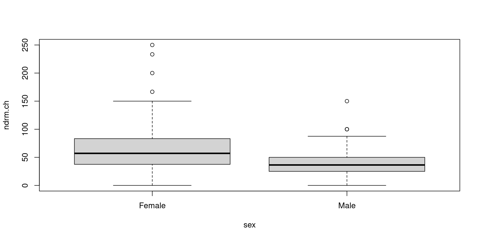
FAMuSS data set: comparing ndrm.ch by sex
Does change in non-dominant arm strength after resistance training differ between men and women?
FAMuSS: comparing ndrm.ch by sex…
FAMuSS: comparing ndrm.ch by sex…
favstats(ndrm.ch ~ sex, data = famuss) sex min Q1 median Q3 max mean sd n missing
1 Female 0 37.5 57.1 83.3 250 62.92720 36.51909 353 0
2 Male 0 25.0 36.4 50.0 150 39.23512 20.60331 242 0Difference of means:
diffmean(ndrm.ch ~ sex, data = famuss) diffmean
-23.69207 The independent two-group \(t\)-test
The null and alternative hypotheses are
-
\(H_0: \mu_F = \mu_M\), the population mean change in arm strength for women is the same as the population mean change in arm strength for men
- Equivalently, \(H_0: \Delta = \mu_F - \mu_M = 0\)
\(H_A: \mu_F \neq \mu_M\), the population mean change in arm strength for women is different from the population mean change in arm strength for men
In general, the hypotheses are written in terms of \(\mu_1\) and \(\mu_2\).
The parameter of interest is \(\mu_1 - \mu_2\).
The point estimate is \(\overline{x}_1 - \overline{x}_2\).
The independent two-group \(t\)-test…
The \(t\)-statistic is:
\[t =\dfrac{ (\overline{x}_{1} - \overline{x}_{2})- (\mu_1 - \mu_2)} {\sqrt{\dfrac{s_1^2}{n_1} + \dfrac{s_2^2}{n_2}}} \]
The \(p\)-value is calculated as usual, but the degrees of freedom for the distribution are different from for the paired data setting…
Degrees of freedom for the independent two-group \(t\)-test
When doing the test by hand, use the following approximation: \[df = \text{min}(n_1 - 1, n_2 - 1) \]
R uses a better approximation, known as the Satterthwaite approximation:
\[df = \dfrac{\left[(s_1^2/n_1) + (s_2^2/n_2)\right]^2}{\left[(s_1^2/n_1)^2/(n_1 - 1) + (s_2^2/n_2)^2/(n_2 - 1)\right]}\]
FAMuSS Example
\(\overline{x}_1 - \overline{x}_2\):
diffmean(ndrm.ch ~ sex, data = famuss) diffmean
-23.69207 Standard deviations:
sd(ndrm.ch ~ sex, data = famuss) Female Male
36.51909 20.60331 Sample sizes:
\(\displaystyle SE = \sqrt{\dfrac{s_1^2}{n_1} + \dfrac{s_2^2}{n_2}}\)
\(\displaystyle t =\dfrac{ (\overline{x}_{1} - \overline{x}_{2})- (\mu_1 - \mu_2)}{SE}\)
\(SE = 2.352051\)
\(t = -10.0729411\)
Two-tailed test p-value:
2 * pt(-10.07, df = 241)[1] 3.904446e-20We have sufficient evidence to reject the null hypothesis that there is no difference in the change of the non-dominant arm strength between males and females, at 5% significance level.
Confidence intervals for independent two-group data
The 95% confidence interval for the difference in population means has the form \[( \overline{x}_{1} - \overline{x}_{2}) \pm \left( t^{\star} \times \sqrt{\frac{s_{1}^{2}}{n_{1}}+\frac{s_{2}^{2}}{n_{2}}} \right), \]
where \(t^{\star}\) is the point on a \(t\) distribution that has area 0.025 to the right, with the same \(df\) as used for calculating the \(p\)-value of the associated test.
FAMuSS Example
\(\overline{x}_1 - \overline{x}_2\):
diffmean(ndrm.ch ~ sex, data = famuss) diffmean
-23.69207 Standard deviations:
sd(ndrm.ch ~ sex, data = famuss) Female Male
36.51909 20.60331 Sample sizes:
\(\displaystyle SE = \sqrt{\dfrac{s_1^2}{n_1} + \dfrac{s_2^2}{n_2}} = 2.352051\)
Critical \(t\)-score:
qt(0.975, df = 241)[1] 1.969856Margin of error:
\(\displaystyle m = 2.35\cdot 1.9698562 = 4.6291621\)
Interval: \(\left( -23.69207 - 4.6291621, -23.69207 + 4.6291621 \right)\)
\({}=\left( -28.3212321, -19.0629079 \right)\)
We are 95% confident that the interval \(\left( -28.321, -19.063 \right)\) contains the population difference between the change of the non-dominant arm strength in males and females.
Letting R do the work
t.test(ndrm.ch ~ sex, data = famuss, mu = 0,
       alternative = "two.sided")
    Welch Two Sample t-test

data:  ndrm.ch by sex
t = 10.073, df = 574.01, p-value < 2.2e-16
alternative hypothesis: true difference in means between group Female and group Male is not equal to 0
95 percent confidence interval:
 19.07240 28.31175
sample estimates:
mean in group Female   mean in group Male
            62.92720             39.23512
Hand calculation produced (using df = 241):
\(t = -10.0729411\)
\(P\)-value: \(3.9044459\times 10^{-20}\)
Interval:
\(\left( -28.321, -19.063 \right)\)
Example (Egg volume)
In a study examining 131 collared flycatcher eggs, researchers measured various characteristics in order to study their relationship to egg size (assayed as egg volume, in \(\text{mm}^3\)). These characteristics included nestling sex and survival. A single pair of collared flycatchers generally lays around 6 eggs per breeding season; laying order of the eggs was also recorded.
Is there evidence at the \(\alpha = 0.10\) significance level to suggest that egg size differs between male and female chicks?
- For male chicks, \(\overline{x} = 1619.95\), \(s = 127.54\), and \(n = 80\).
- For female chicks, \(\overline{x} = 1584.20\), \(s = 102.51\), and \(n = 48\).
Sex was only recorded for eggs that hatched.
T-Table

Example (Egg volume)
In a study examining 131 collared flycatcher eggs, researchers measured various characteristics in order to study their relationship to egg size (assayed as egg volume, in \(\text{mm}^3\)). These characteristics included nestling sex and survival. A single pair of collared flycatchers generally lays around 6 eggs per breeding season; laying order of the eggs was also recorded.
Construct a 95% confidence interval for the difference in egg size between chicks that successfully fledged (developed capacity to fly) and chicks that died in the nest. From the interval, is there evidence of a size difference in eggs between these two groups?
- For chicks that fledged, \(\overline{x} = 1605.87\), \(s = 126.32\), and \(n = 89\).
- For chicks that died in the nest, \(\overline{x} = 1606.91\), \(s = 103.46\), \(n = 42\).
Comparison of the two designs
Within subjects design is more powerful (it is easier to reject a false null hypothesis, confidence intervals have smaller margins of error).
It is not always possible, for example when you are comparing two treatments (poisoning the well).