Math 132B

Class 22

FAMuSS Study

We saw the “FAMuSS” data in part 2, when we were trying to answer the question

Is change in non-dominant arm strength after resistance training associated with sex?

We had two populations: females and males, and we wanted to know if the mean change in non-dominant arm strength is different in these two populations.

This was an example of inference about means of two independent populations.

The main question of the FAMuSS study, however, was

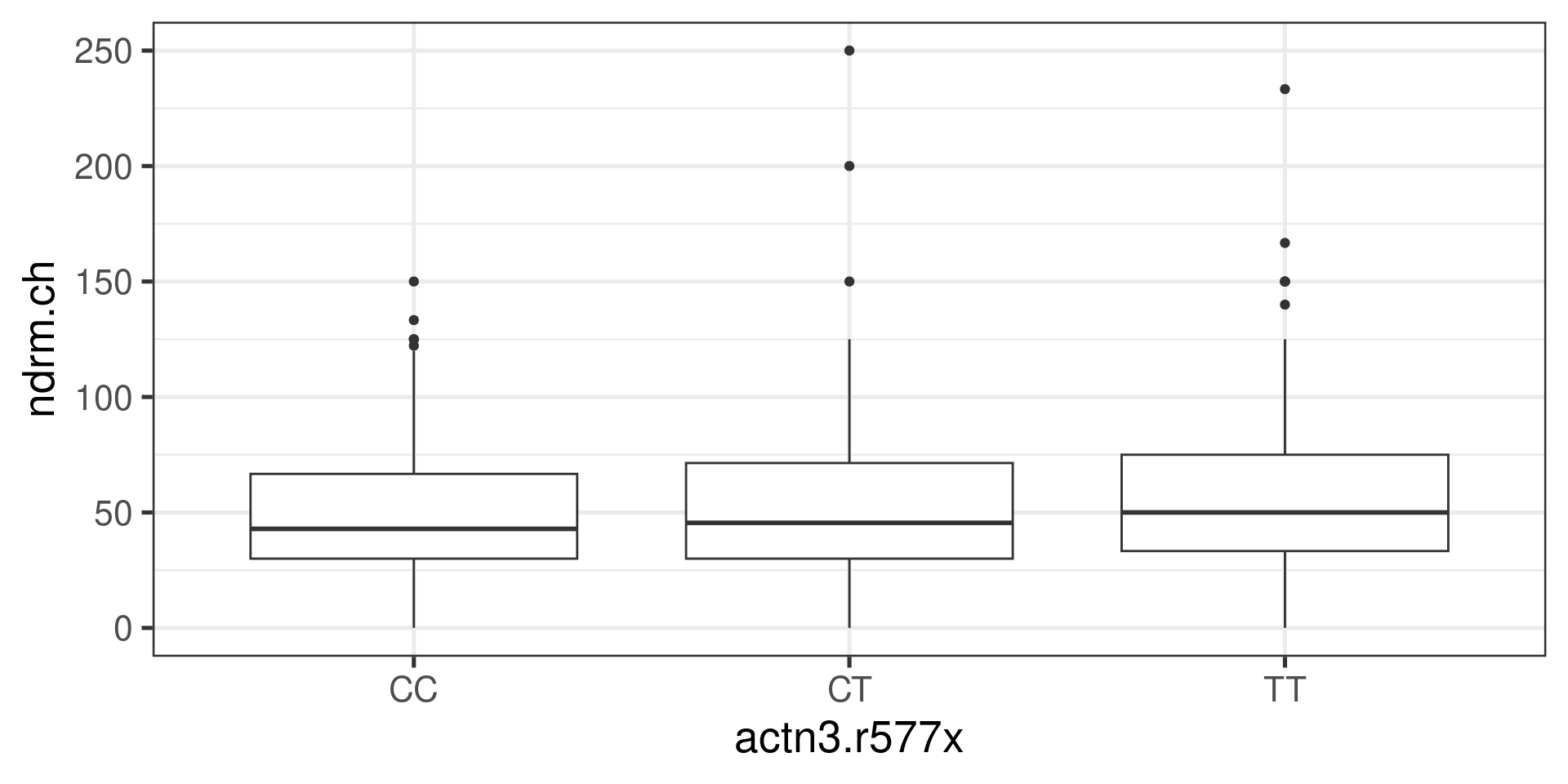
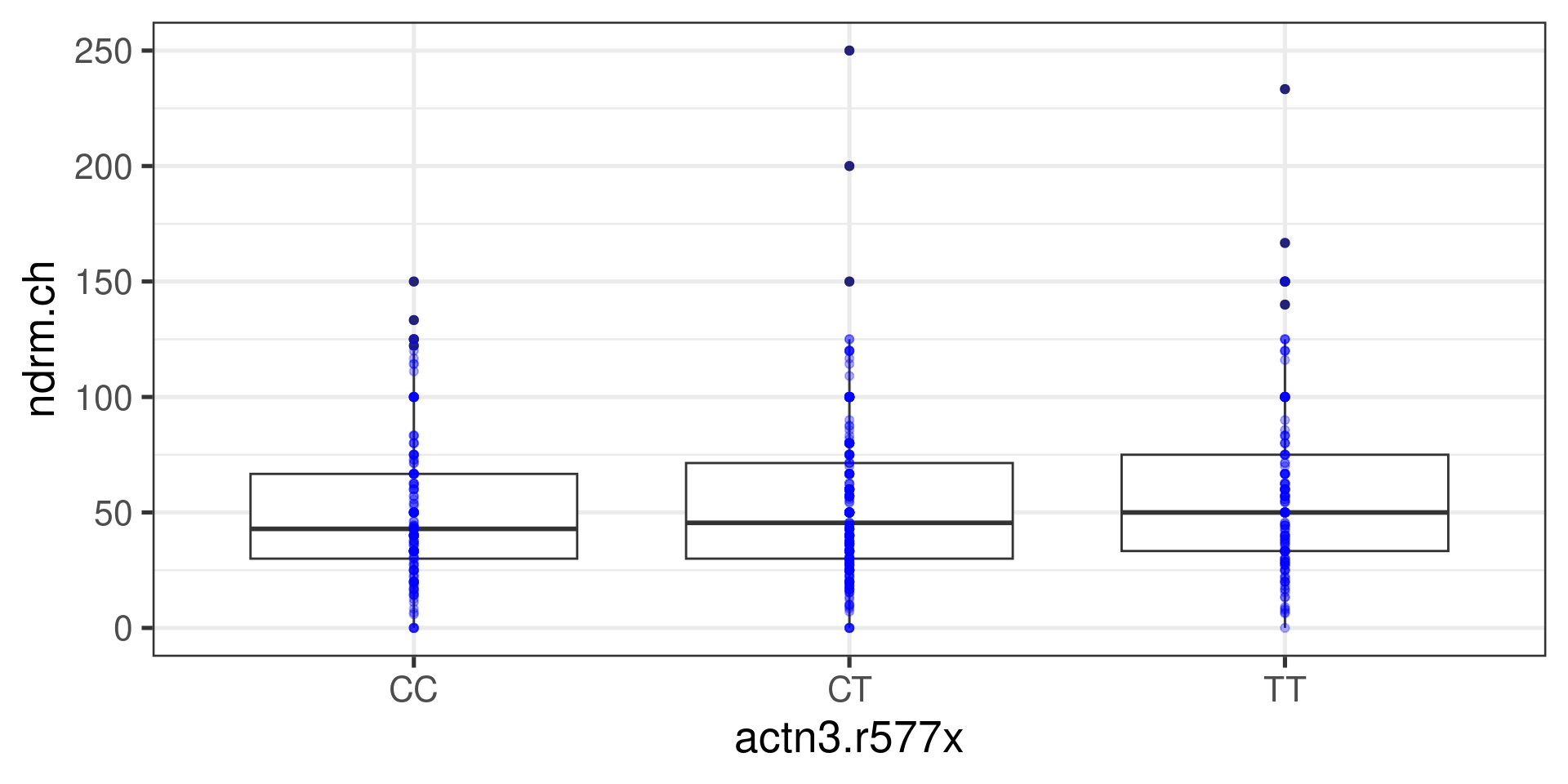
Is change in non-dominant arm strength after resistance training associated with ACTN3 (R577X polymorphism) genotype?

How many genotypes are there?

FAMuSS Data

Rows: 595
Columns: 9
$ ndrm.ch     <dbl> 40.0, 25.0, 40.0, 125.0, 40.0, 75.0, 100.0, 57.1…
$ drm.ch      <dbl> 40.0, 0.0, 0.0, 0.0, 20.0, 0.0, 0.0, -14.3, 0.0,…
$ sex         <fct> Female, Male, Female, Female, Female, Female, Fe…
$ age         <int> 27, 36, 24, 40, 32, 24, 30, 28, 27, 30, 20, 23, …
$ race        <fct> Caucasian, Caucasian, Caucasian, Caucasian, Cauc…
$ height      <dbl> 65.0, 71.7, 65.0, 68.0, 61.0, 62.2, 65.0, 68.0, …
$ weight      <dbl> 199, 189, 134, 171, 118, 120, 134, 162, 189, 120…
$ actn3.r577x <fct> CC, CT, CT, CT, CC, CT, TT, CT, CC, CT, CT, CT, …
$ bmi         <dbl> 33.112, 25.845, 22.296, 25.998, 22.293, 21.805, …

Levels of actn3.r577x:

levels(famuss$actn3.r577x)

[1] "CC" "CT" "TT"

FAMuSS Data

Back to two independent groups

The question was: Is there an association between the variable sex (categorical with two levels) and the variable ndrm.ch (numerical)?

We calculated the difference of the means of the two groups:

diffmean(ndrm.ch ~ sex, data = famuss)

 diffmean 
-23.69207

We wanted to know if this is a small difference or a large difference.

Central Limit Theorem

We knew that under some assumptions, if the null hypothesis \(H_0: \mu_1 - \mu_2 = 0\), the quantity \[t = \frac{\overline{x}_1 - \overline{x}_2}{\sqrt{\frac{s_1^2}{n_1} + \frac{s_2^2}{n_2}}}\] (\(t\)-statistic) is distributed according to the \(T\) distribution with some known number of degrees of freedom.

We asked “how likely would it be, assuming the null hypothesis is true, to have a \(t\)-statistic like the observed one or more extreme” (\(p\)-value)?”

In other words: “How well does the null model explain the observed difference?”

There is a simpler way.

Permutation test

What kind of difference in means would we get if the values of ndrm.ch were assigned to the two sex categories completely randomly?

diffmean(shuffle(ndrm.ch) ~ sex, data = famuss)

  diffmean 
-0.7344298

Do it many times:

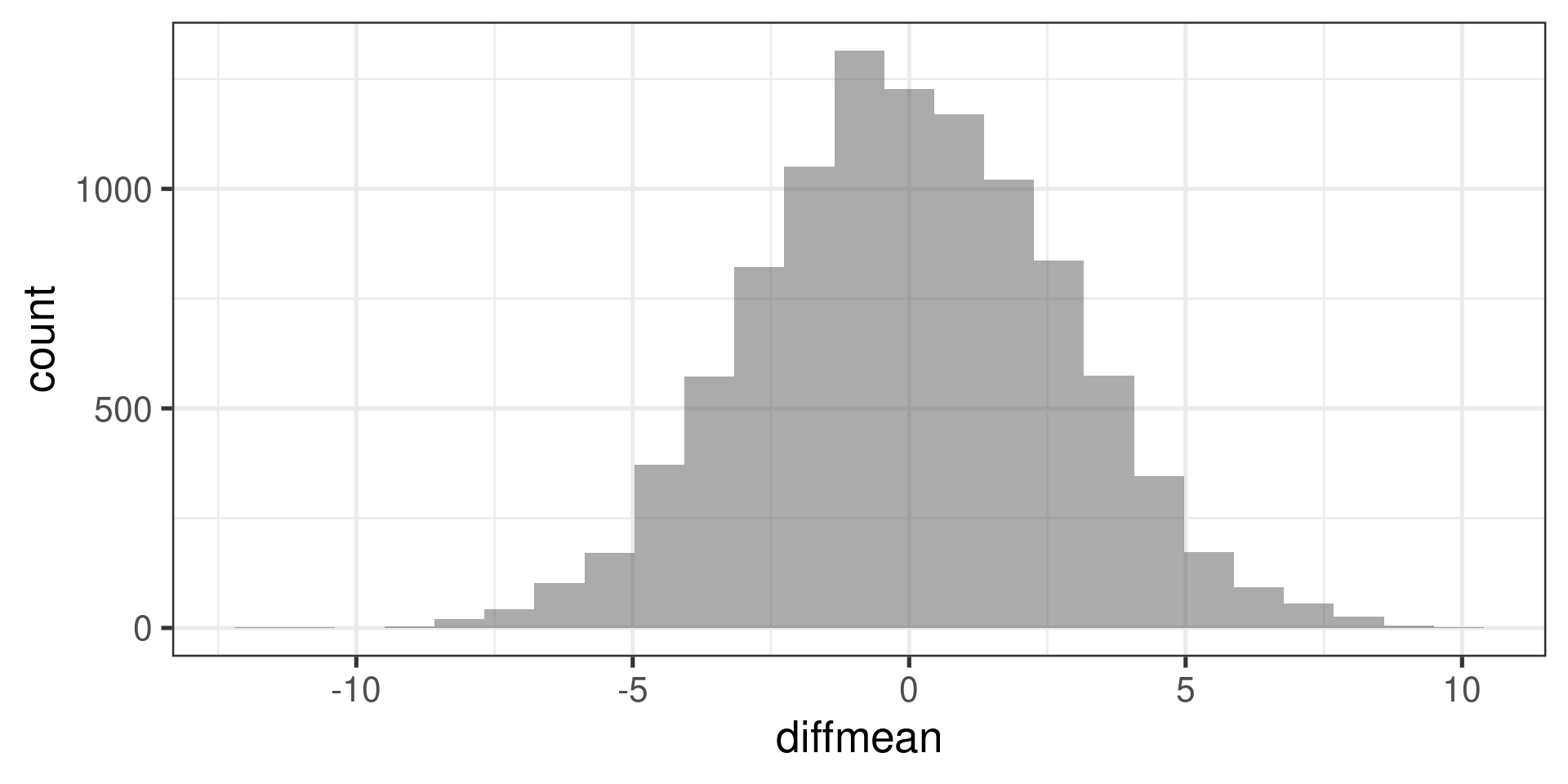
do(10000) * diffmean(shuffle(ndrm.ch) ~ sex, data = famuss) -> perms

What do we get

and where does -23.6920715 (the observed difference) fit into it?

Back to multiple groups

The question is now: Is there an association between the variable actn3.r577x (categorical with more than two levels) and the variable ndrm.ch (numerical)?

We could do a permutation test, but what number are we going to calculate?

In other words: What should be the test statistic?

Analysis of Variance (ANOVA)

We are interested in comparing means across more than two groups.

Why not conduct several two-sample \(t\)-tests?

If there are \(k\) groups, then \({k \choose 2} = \frac{k(k-1)}{2}\) \(t\)-tests are needed.
Conducting multiple tests on the same data increases the overall rate of Type I error.

ANOVA uses a single hypothesis test to assess whether means across many groups are equal:

\(H_0\): mean outcome is same across all groups (\(\mu_1 = \mu_2 = \mu_3 = ... = \mu_k\))
\(H_A\): at least one mean is different from the others (i.e., means are not all equal)

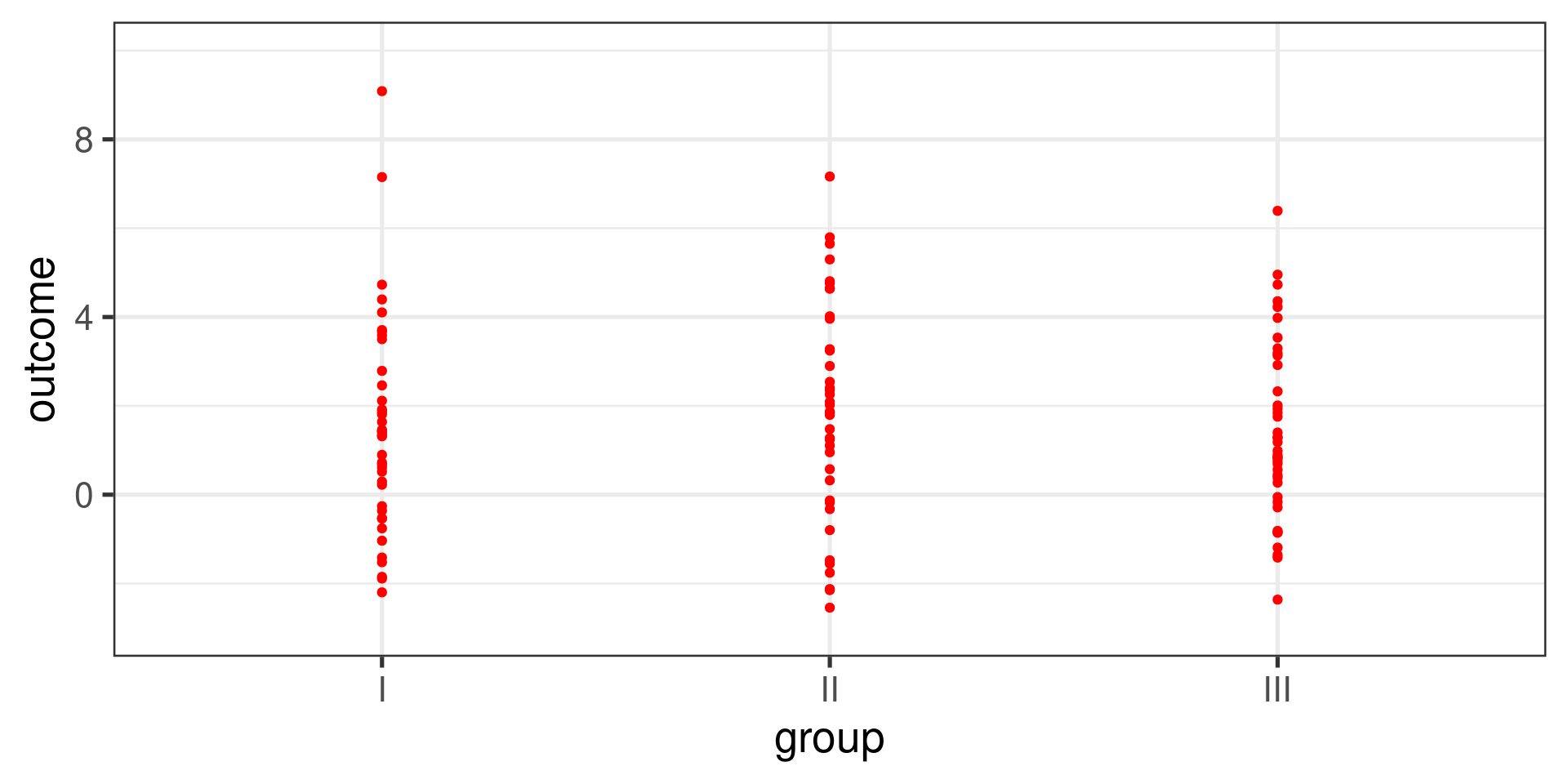
Are the means equal?

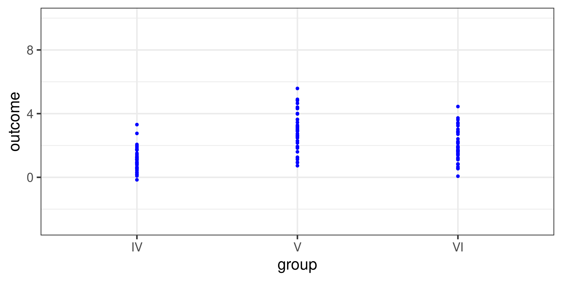
Idea behind ANOVA

Is the variability in the sample means large enough that it seems unlikely to be from chance alone?

Compare two quantities:

Variability between groups (Mean Square between Groups, or \(MSG\)):
- How different are the group means from each other?
- How much does each group mean vary from the overall mean?

Variability within groups (Mean Square Error, or \(MSE\)):
- How variable are the data within each group?

The \(F\) statistic is the ratio of \(MSG\) to \(MSE\).

Formulas

Mean Square between Groups:

\[MSG = \frac{1}{k-1}\sum_{i=1}^{k} n_{i}\left(\overline{x}_{i} - \overline{x}\right)^{2}\]
Mean Square Error:

\[MSE = \frac{1}{n-k}\sum_{i=1}^{k} (n_i-1)s_i^{2}\]
The F Statistic

\[F = \frac{MSG}{MSE}\]

Where:

\(k\) is the number of groups
\(n\) is the overall sample size

\[n = \sum_{i=1}^k n_i\]
\(\overline{x}\) is the overall mean of \(x\)
\(n_i\) is the size of \(i\)-th group
\(\overline{x}_i\) is the mean of \(i\)-th group
\(s_i\) is the standard deviation of \(i\)-th group

FAMuSS Example

Overall statistics:

 min Q1 median   Q3 max     mean       sd   n missing
   0 30   45.5 66.7 250 53.29109 33.13923 595       0

Statistics by group:

  actn3.r577x min   Q1 median   Q3   max     mean       sd   n missing
1          CC   0 30.0   42.9 66.7 150.0 48.89422 29.95608 173       0
2          CT   0 30.0   45.5 71.4 250.0 53.24904 33.23148 261       0
3          TT   0 33.3   50.0 75.0 233.3 58.08385 35.69133 161       0

Calculation

Mean Square between Groups:

\[MSG = \frac{1}{k-1}\sum_{i=1}^{k} n_{i}\left(\overline{x}_{i} - \overline{x}\right)^{2}\]
Mean Square Error:

\[MSE = \frac{1}{n-k}\sum_{i=1}^{k} (n_i-1)s_i^{2}\]
The F Statistic

\[F = \frac{MSG}{MSE}\]
Is this small, large or normal?

Let the computer do it:

xbar <- mean(~ndrm.ch, data = famuss)
famuss |>
    group_by(actn3.r577x) |>
    summarize(
        xibar = mean(ndrm.ch),
        si = sd(ndrm.ch),
        ni = n()
    ) |>
    mutate(xibar_minus_xbar = xibar - xbar) |>
    summarize(
        k = n(),
        MSG = sum(ni * xibar_minus_xbar^2) / (k - 1),
        MSE = sum((ni - 1) * si^2) / (sum(ni) - k),
        F = MSG/MSE
    )

Let the computer do it:

# A tibble: 1 × 4
      k   MSG   MSE     F
  <int> <dbl> <dbl> <dbl>
1     3 3522. 1090.  3.23

With no association

famuss |>
    group_by(shuffle(actn3.r577x)) |>
    summarize(
        xibar = mean(ndrm.ch),
        si = sd(ndrm.ch),
        ni = n()
    ) |>
    mutate(xibar_minus_xbar = xibar - xbar) |>
    summarize(
        k = n(),
        MSG = sum(ni * xibar_minus_xbar^2) / (k - 1),
        MSE = sum((ni - 1) * si^2) / (sum(ni) - k),
        F = MSG/MSE
    )

With no association

# A tibble: 1 × 4
      k   MSG   MSE     F
  <int> <dbl> <dbl> <dbl>
1     3 1036. 1098. 0.943

Repeat many times

do(10000) * {
    famuss |>
        group_by(shuffle(actn3.r577x)) |>
        summarize(
            xibar = mean(ndrm.ch),
            si = sd(ndrm.ch),
            ni = n()
        ) |>
        mutate(xibar_minus_xbar = xibar - xbar) |>
        summarize(
            k = n(),
            MSG = sum(ni * xibar_minus_xbar^2) / (k - 1),
            MSE = sum((ni - 1) * si^2) / (sum(ni) - k),
            F = MSG/MSE
        )
    } -> F_stats

Results

Rows: 10,000
Columns: 4
$ k   <int> 3, 3, 3, 3, 3, 3, 3, 3, 3, 3, 3, 3, 3, 3, 3, 3, 3, 3, 3, 3, 3, 3, …
$ MSG <dbl> 591.92542, 1326.37761, 1017.32145, 130.96503, 492.63014, 2756.3682…
$ MSE <dbl> 1099.919, 1097.438, 1098.482, 1101.476, 1100.254, 1092.607, 1100.1…
$ F   <dbl> 0.53815373, 1.20861326, 0.92611599, 0.11889956, 0.44774207, 2.5227…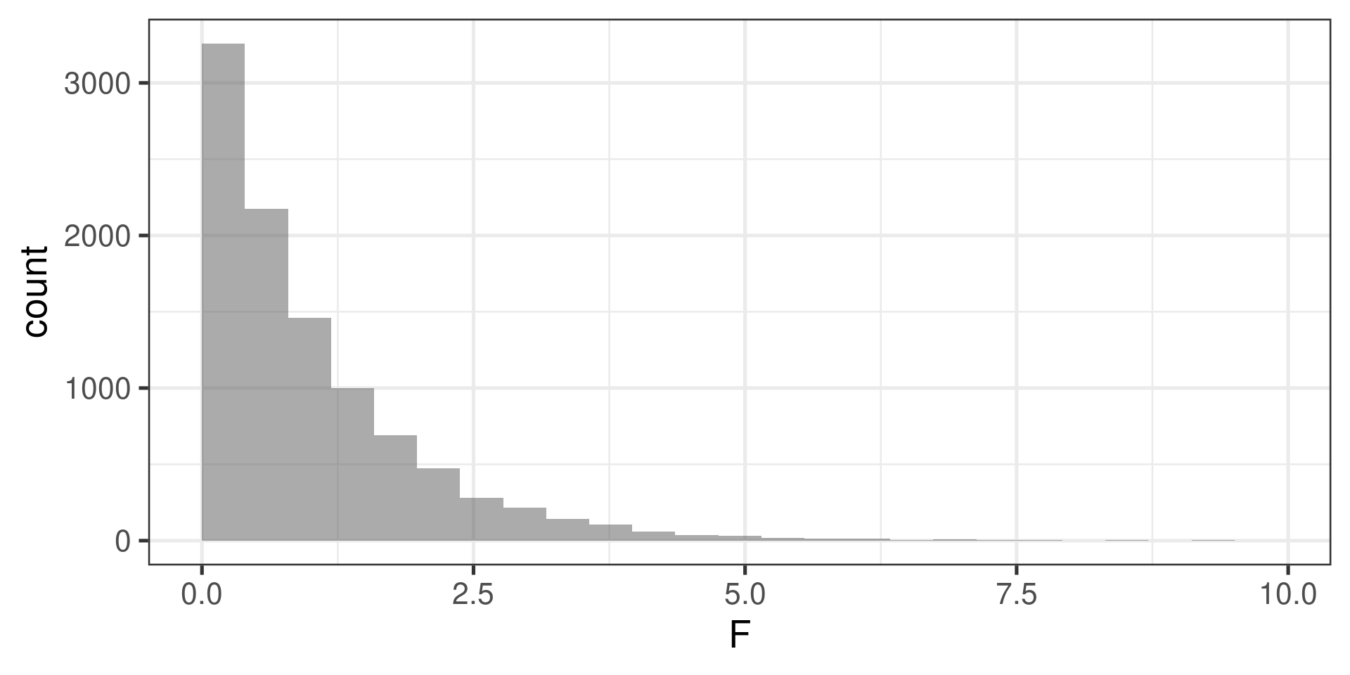

Compare observed value with the null distribution

The observed value was 3.23.
In what proportion of the repetition was the F-statistic higher than 3.23?

prop(~(F > 3.23), data = F_stats)

prop_TRUE 
   0.0411

Meaning of F-statistic

The null hypothesis says that there is no real difference between the groups; thus, any observed variation in group means is due to chance.

Think of all observations as belonging to a single group.
Variability between group means should equal variability within groups

The F-statistic is the test statistic for ANOVA.

\[F = \frac{\text{variance between groups}}{\text{variance within groups}} = \frac{MSG}{MSE}\]

When the population means are equal, the \(F\)-statistic is approximately 1 or less than 1.
When the population means differ, \(F\) will be larger than 1. Larger values of \(F\) represent stronger evidence against the null.

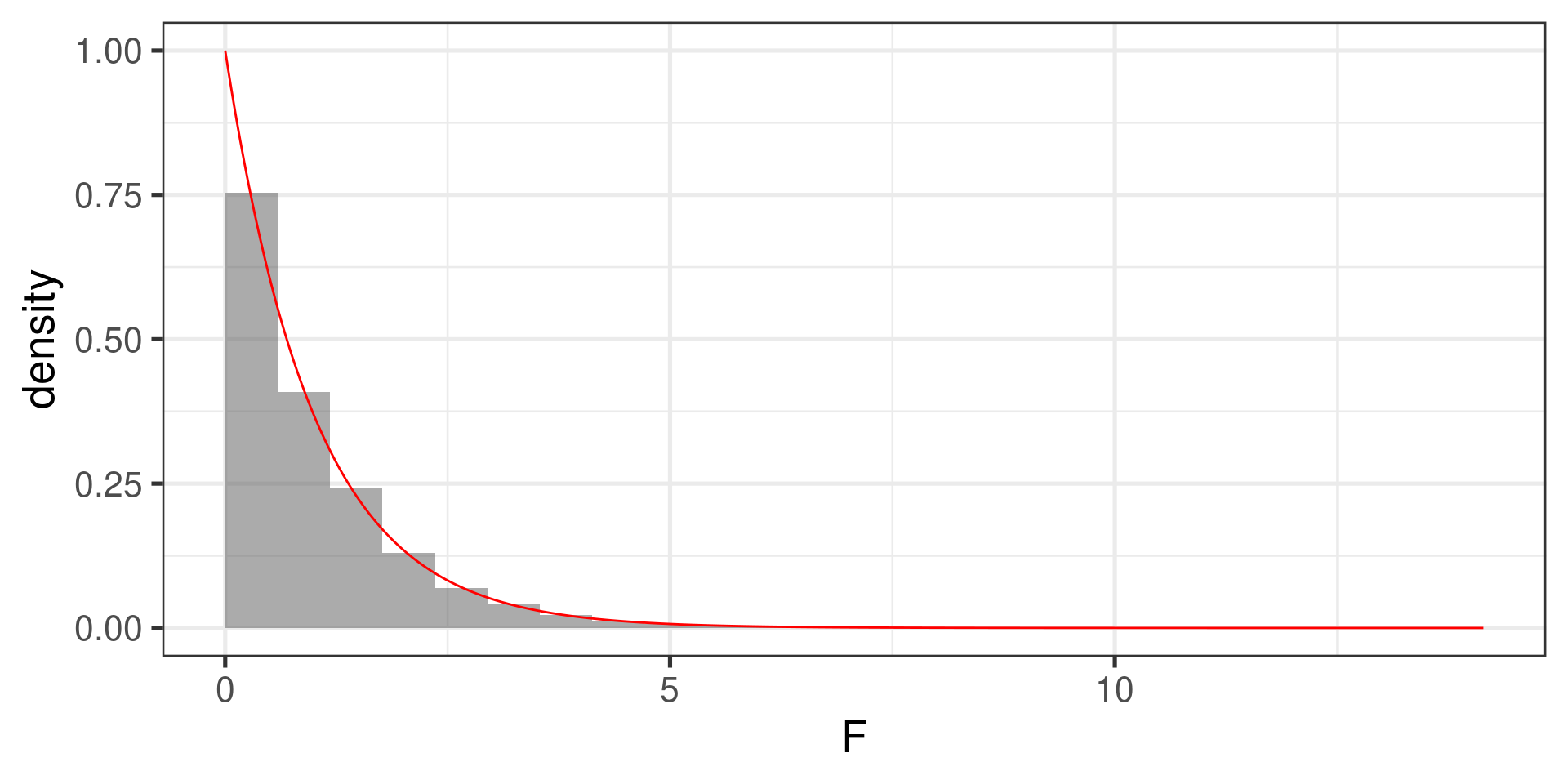
F-distribution

The \(F\) statistic follows n \(F\) distribution, with two degrees of freedom, \(df_1\) and \(df_2\):
- \(df_1 = n_{groups} - 1 = k - 1\) (also known as numerator df)
- \(df_2 = n_{obs} - n_{groups} = n - k\) (also known as denominator df).
The \(p\)-value for the \(F\)-statistic is the probability \(F\) statistic of a sample from a population in which \(H_0\) is true is larger than the observed \(F\)-statistic.
It is the area to the right of the observed F-statistic under the F-curve with \(df_1 = k - 1\) and \(df_2 = n - k\).

1 - pf(3.23, df1 = 3 - 1, df2 = 595 - 3)

[1] 0.04025569

Plot of F-Distribution

Letting R do all the work

anova(lm(ndrm.ch ~ actn3.r577x, data = famuss))

Analysis of Variance Table

Response: ndrm.ch
             Df Sum Sq Mean Sq F value  Pr(>F)  
actn3.r577x   2   7043  3521.6  3.2308 0.04022 *
Residuals   592 645293  1090.0                  
---
Signif. codes:  0 '***' 0.001 '**' 0.01 '*' 0.05 '.' 0.1 ' ' 1

Assumptions for ANOVA

It is important to check whether the assumptions for conducting ANOVA are reasonably satisfied:

Observations independent within and across groups
- Think about study design/context
Data within each group are nearly normal
- Look at the data graphically, such as with a histogram
- Normal Q-Q plots can help…
Variability across groups is about equal
- Look at the data graphically
- Numerical rule of thumb: ratio of largest variance to smallest variance < 3 is considered “about equal”

Histograms

gf_histogram(~ndrm.ch | actn3.r577x, data = famuss)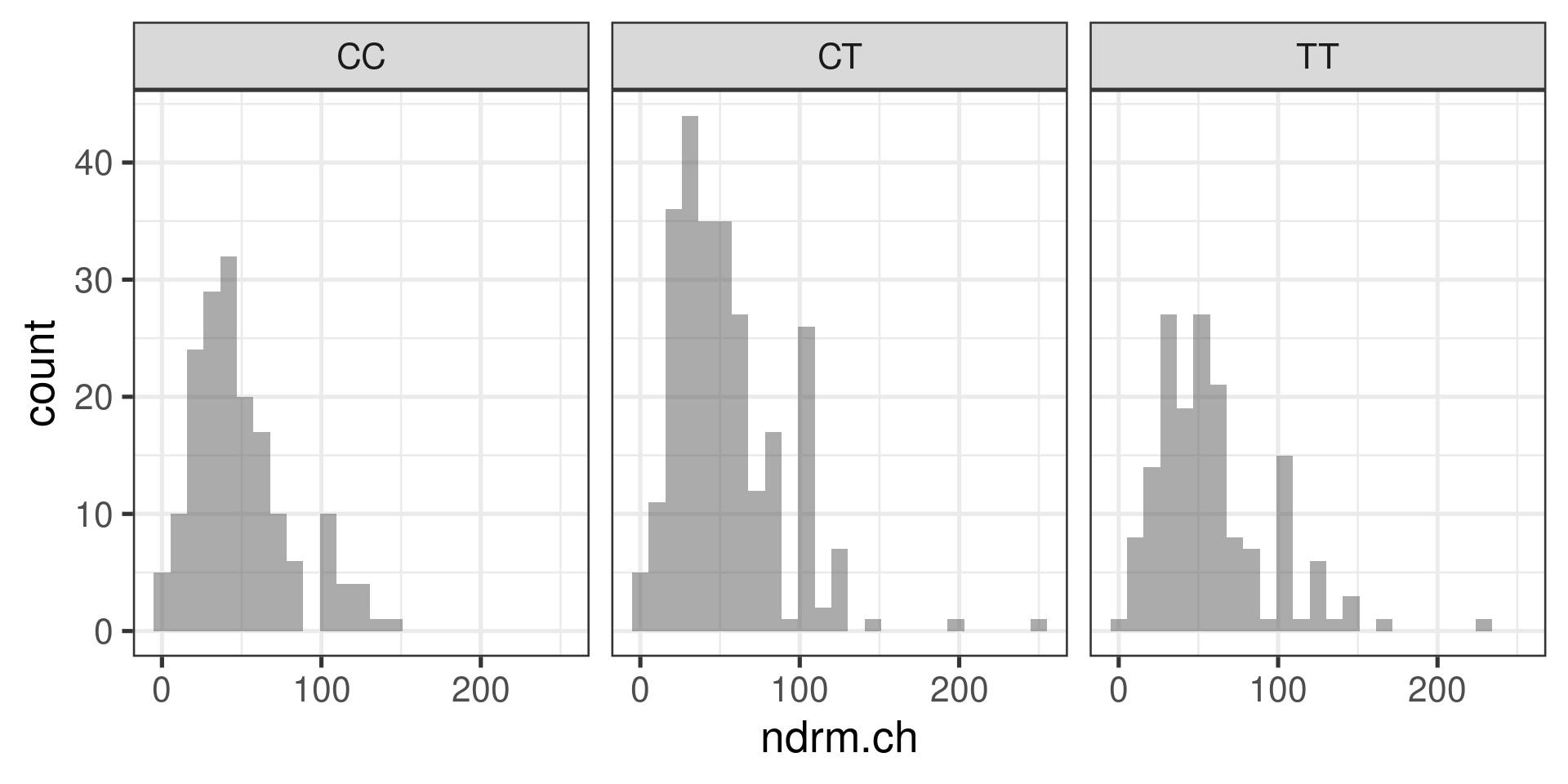

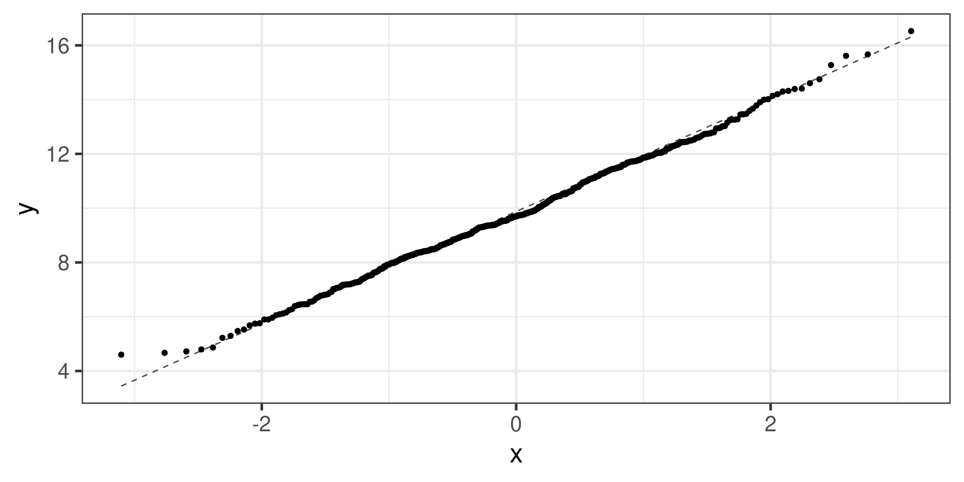
Normal probability plots (Q-Q plots)

gf_qq(~ndrm.ch | actn3.r577x,  data = famuss) |>
    gf_qqline()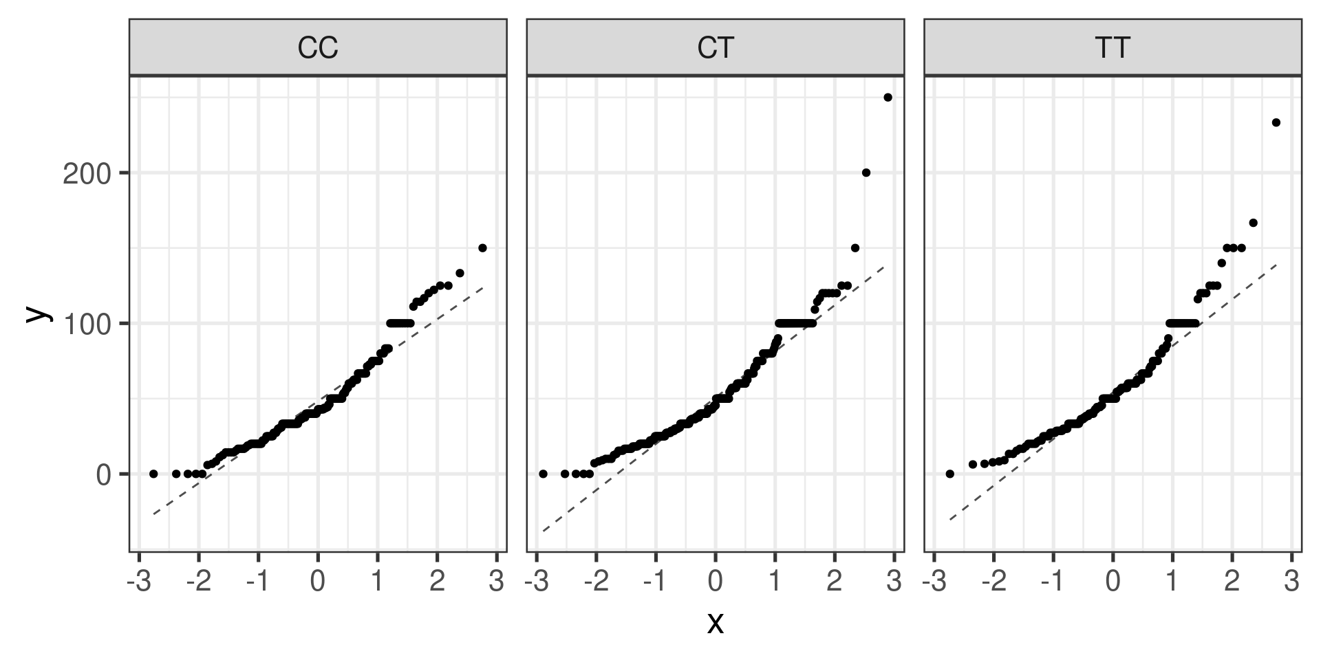

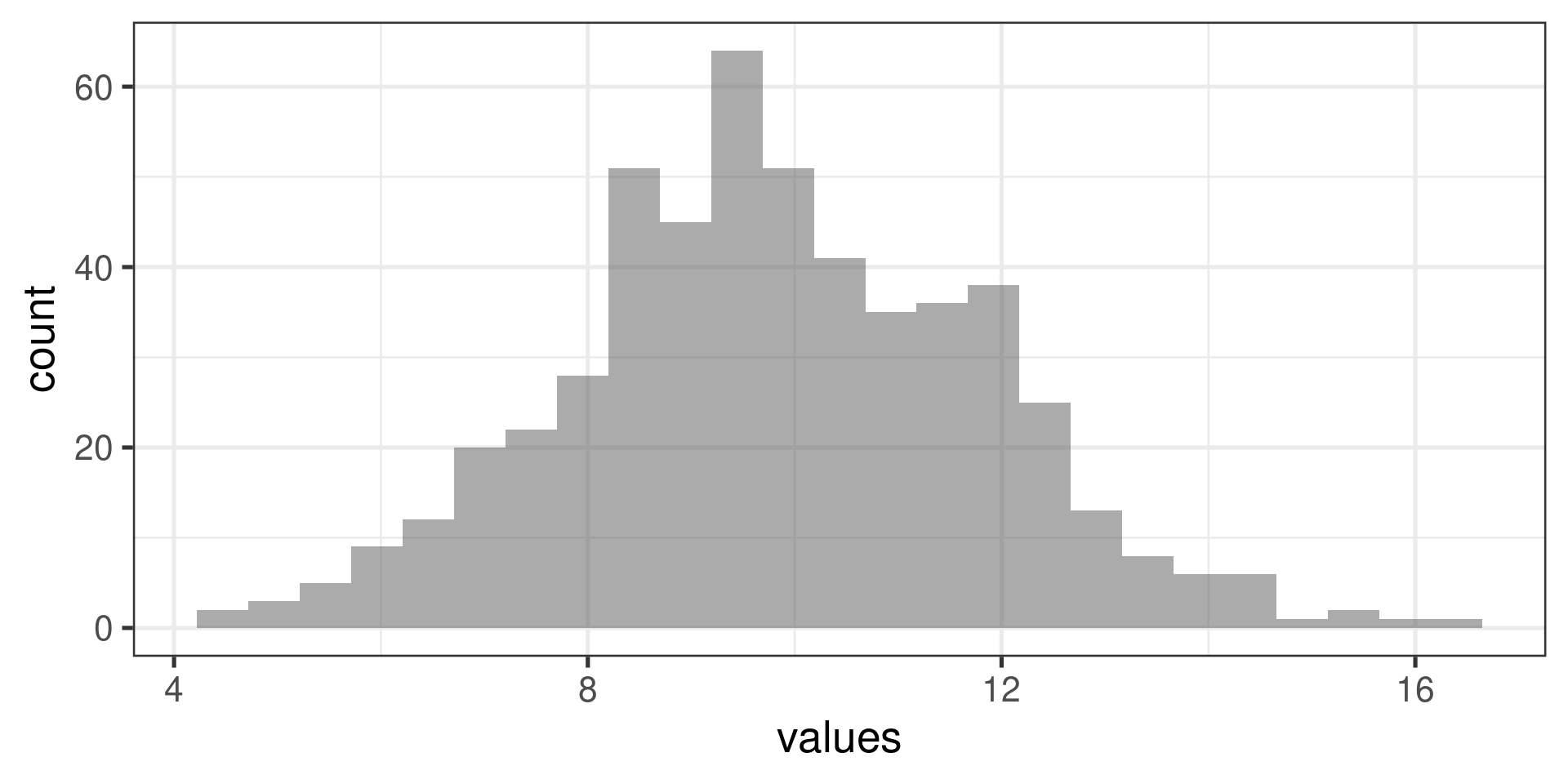
Normal probability plots examples

Right skewed distribution:

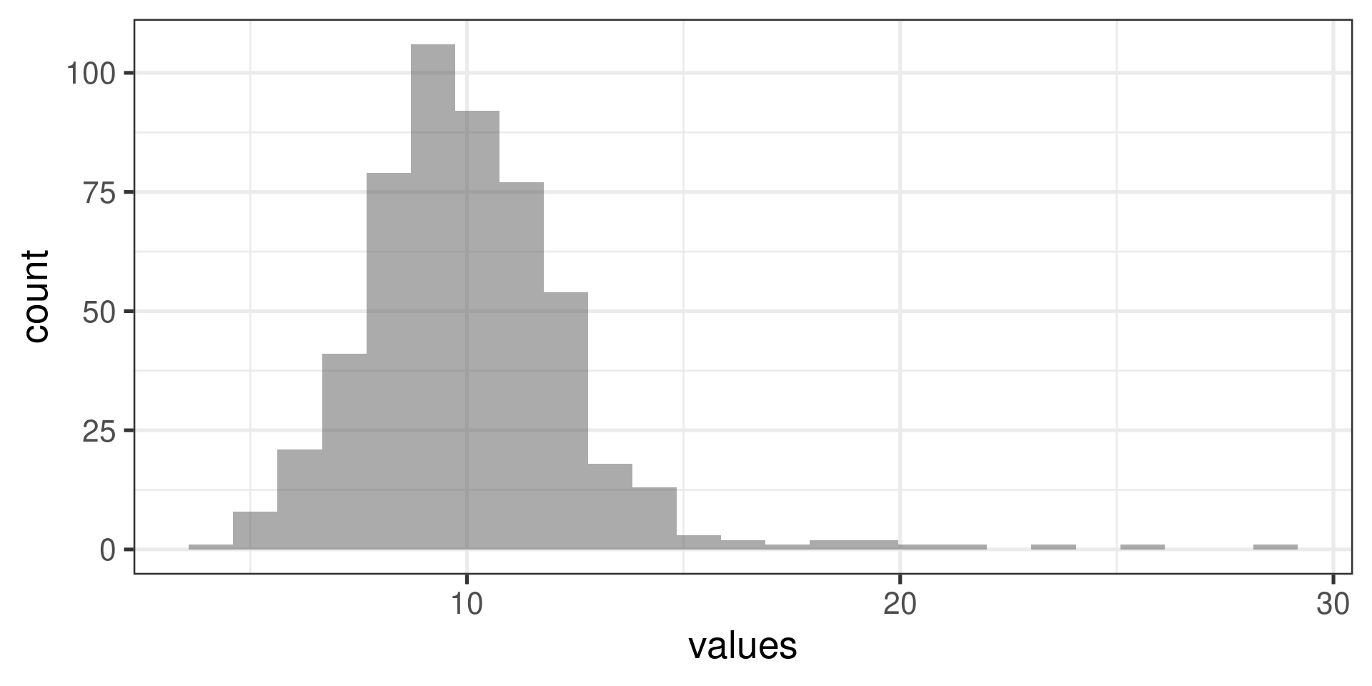
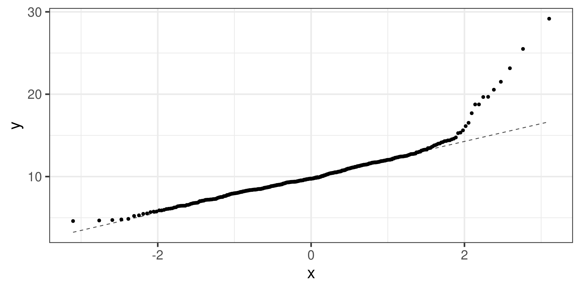
Normal probability plots examples

“Uniform” distribution:

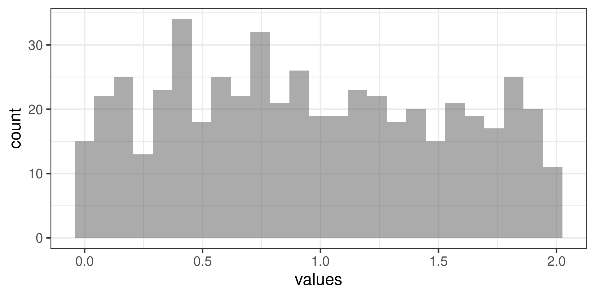
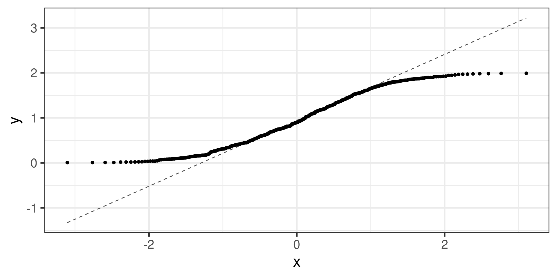
Normal probability plots examples

Normal distribution: