Math 132B

Class 23

FAMuSS Study

The main question of the FAMuSS study was

Is change in non-dominant arm strength after resistance training associated with ACTN3 (R577X polymorphism) genotype?

Rows: 595
Columns: 9
$ ndrm.ch     <dbl> 40.0, 25.0, 40.0, 125.0, 40.0, 75.0, 100.0, 57.1…
$ drm.ch      <dbl> 40.0, 0.0, 0.0, 0.0, 20.0, 0.0, 0.0, -14.3, 0.0,…
$ sex         <fct> Female, Male, Female, Female, Female, Female, Fe…
$ age         <int> 27, 36, 24, 40, 32, 24, 30, 28, 27, 30, 20, 23, …
$ race        <fct> Caucasian, Caucasian, Caucasian, Caucasian, Cauc…
$ height      <dbl> 65.0, 71.7, 65.0, 68.0, 61.0, 62.2, 65.0, 68.0, …
$ weight      <dbl> 199, 189, 134, 171, 118, 120, 134, 162, 189, 120…
$ actn3.r577x <fct> CC, CT, CT, CT, CC, CT, TT, CT, CC, CT, CT, CT, …
$ bmi         <dbl> 33.112, 25.845, 22.296, 25.998, 22.293, 21.805, …

Levels of actn3.r577x:

levels(famuss$actn3.r577x)

[1] "CC" "CT" "TT"

FAMuSS Study

We had multiple groups

The question was: Is there an association between the variable actn3.r577x (categorical with more than two levels) and the variable ndrm.ch (numerical)?

We calculated the F Statistic:

\[F = \frac{MSG}{MSE}\]

where

\[MSG = \frac{1}{k-1}\sum_{i=1}^{k} n_{i}\left(\overline{x}_{i} - \overline{x}\right)^{2}\]

\[MSE = \frac{1}{n-k}\sum_{i=1}^{k} (n_i-1)s_i^{2}\]

FAMuSS Example

MSG <- 1 / 2 * sum(
    tally(~actn3.r577x, data = famuss) * (
        mean(~ ndrm.ch | actn3.r577x, data = famuss) -
        mean(~ndrm.ch, data = famuss)
    )^2
)

\[MSG = \frac{1}{k-1}\sum_{i=1}^{k} n_{i}\left(\overline{x}_{i} - \overline{x}\right)^{2}\]

[1] 3521.619

MSE <- 1/(nrow(famuss) - 3) * sum(
    (tally(~actn3.r577x, data = famuss) - 1) *
    sd(~ndrm.ch | actn3.r577x, data = famuss)^2
)

\[MSE = \frac{1}{n-k}\sum_{i=1}^{k} (n_i-1)s_i^{2}\]

[1] 1090.021

Fstat <- MSG/MSE

\[F = \frac{MSG}{MSE}\]

[1] 3.23078

Or, what we did

xbar <- mean(~ndrm.ch, data = famuss)
famuss |>
    group_by(actn3.r577x) |>
    summarize(
        xibar = mean(ndrm.ch),
        si = sd(ndrm.ch),
        ni = n()
    ) |>
    mutate(xibar_minus_xbar = xibar - xbar) |>
    summarize(
        k = n(),
        MSG = sum(ni * xibar_minus_xbar^2) / (k - 1),
        MSE = sum((ni - 1) * si^2) / (sum(ni) - k),
        F = MSG/MSE
    )

Or, what we did

# A tibble: 1 × 4
      k   MSG   MSE     F
  <int> <dbl> <dbl> <dbl>
1     3 3522. 1090.  3.23

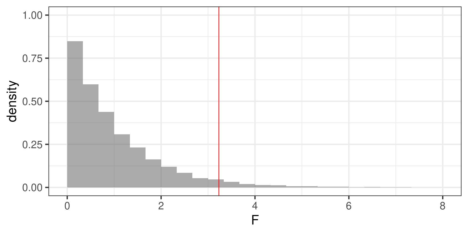
Simulated null distribution

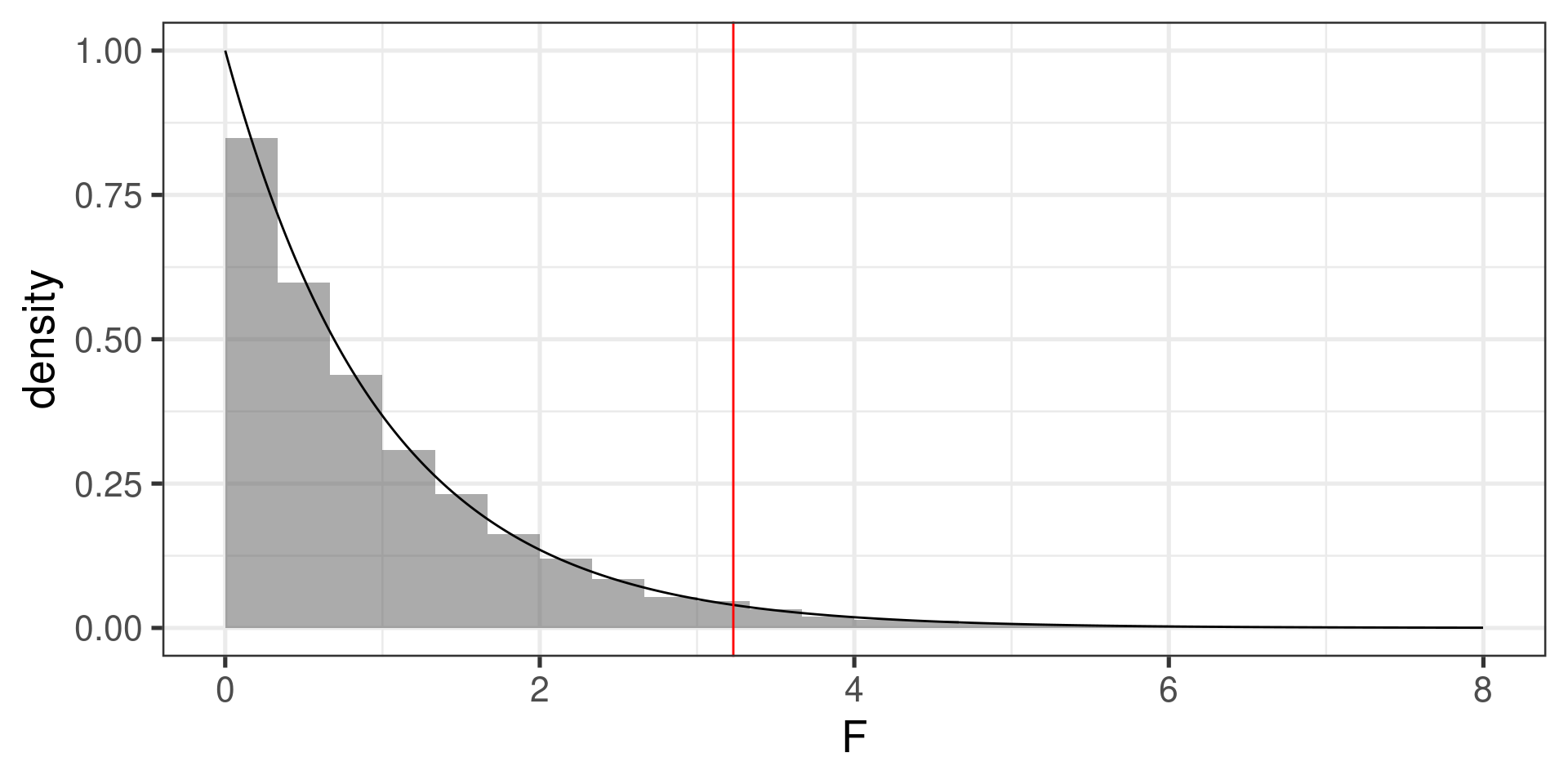
The $p$-value

Simulated:

prop(~(F > 3.23), data = F_stats)

prop_TRUE 
   0.0405

Theoretical:

1 - pf(3.23, df1 = 3 - 1, df2 = 595 - 3)

[1] 0.04025569

Letting R do all the work

anova(lm(ndrm.ch ~ actn3.r577x, data = famuss))

Analysis of Variance Table

Response: ndrm.ch
             Df Sum Sq Mean Sq F value  Pr(>F)  
actn3.r577x   2   7043  3521.6  3.2308 0.04022 *
Residuals   592 645293  1090.0                  
---
Signif. codes:  0 '***' 0.001 '**' 0.01 '*' 0.05 '.' 0.1 ' ' 1

At 5% significance level, We have sufficient evidence that the three population means are not all the same.

Assumptions for ANOVA

It is important to check whether the assumptions for conducting ANOVA are reasonably satisfied:

Observations independent within and across groups
- Think about study design/context
Data within each group are nearly normal
- Look at the data graphically, such as with a histogram
- Normal Q-Q plots can help…
Variability across groups is about equal
- Look at the data graphically
- Numerical rule of thumb: ratio of largest variance to smallest variance < 3 is considered “about equal”

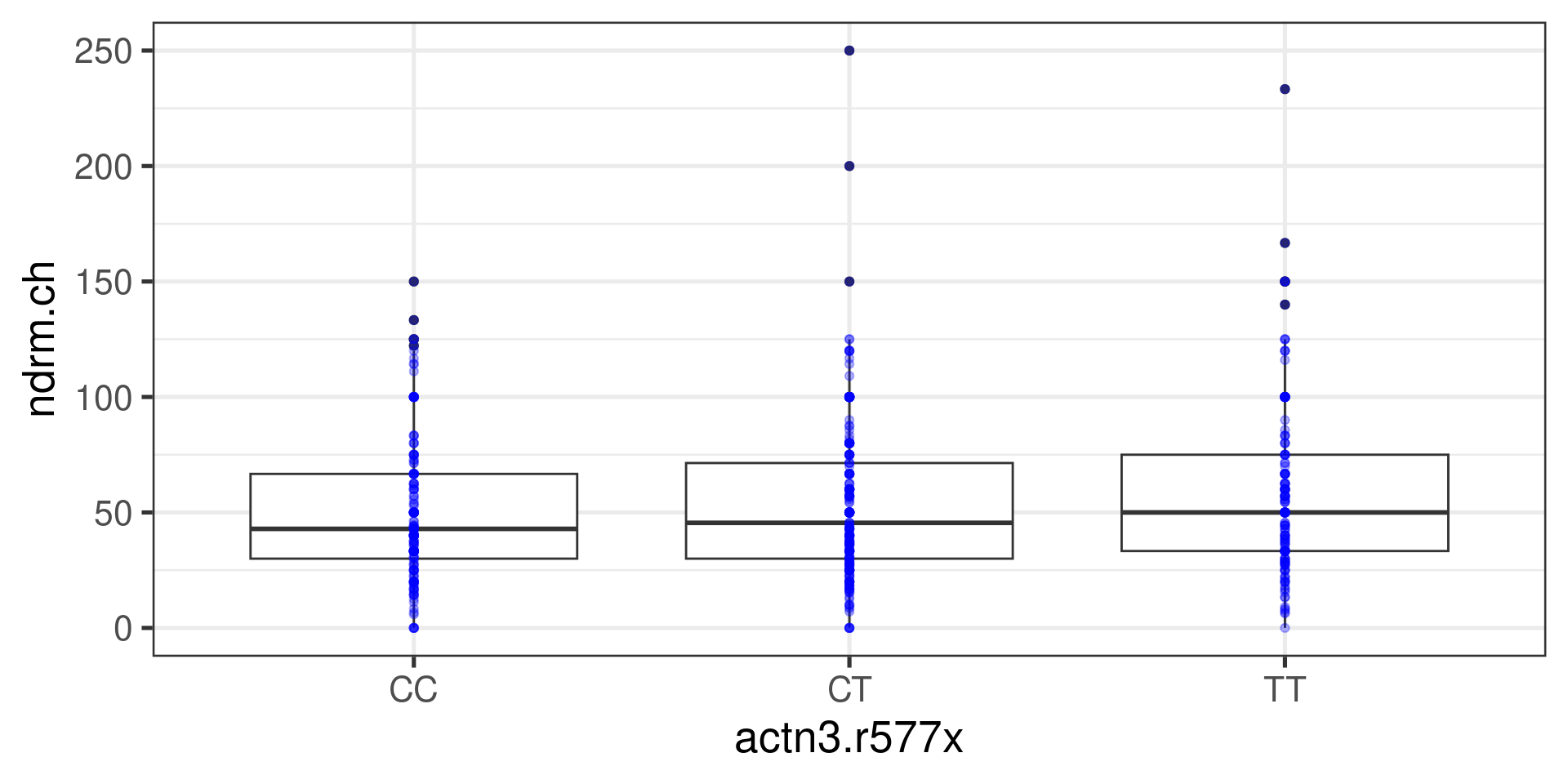
var(ndrm.ch ~ actn3.r577x, data = famuss)

       CC        CT        TT 
 897.3667 1104.3311 1273.8712

Boxplots

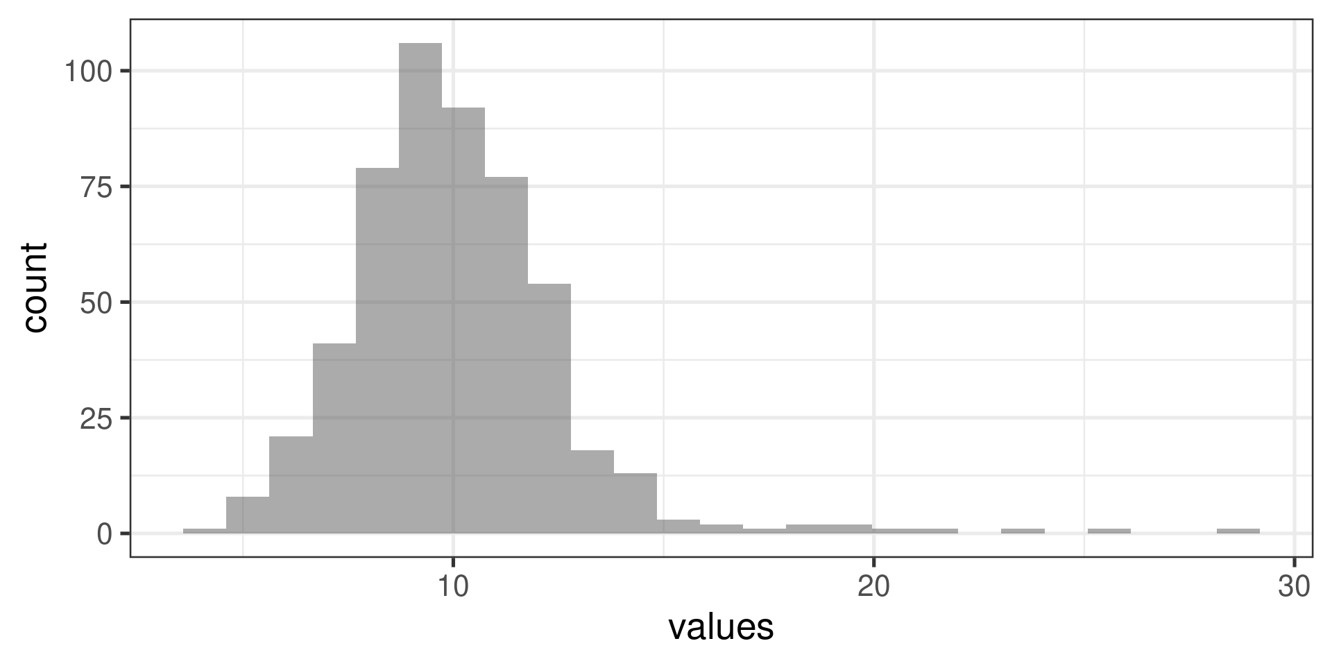
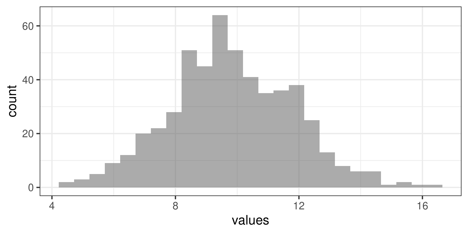
Histograms

gf_histogram(~ndrm.ch | actn3.r577x, data = famuss)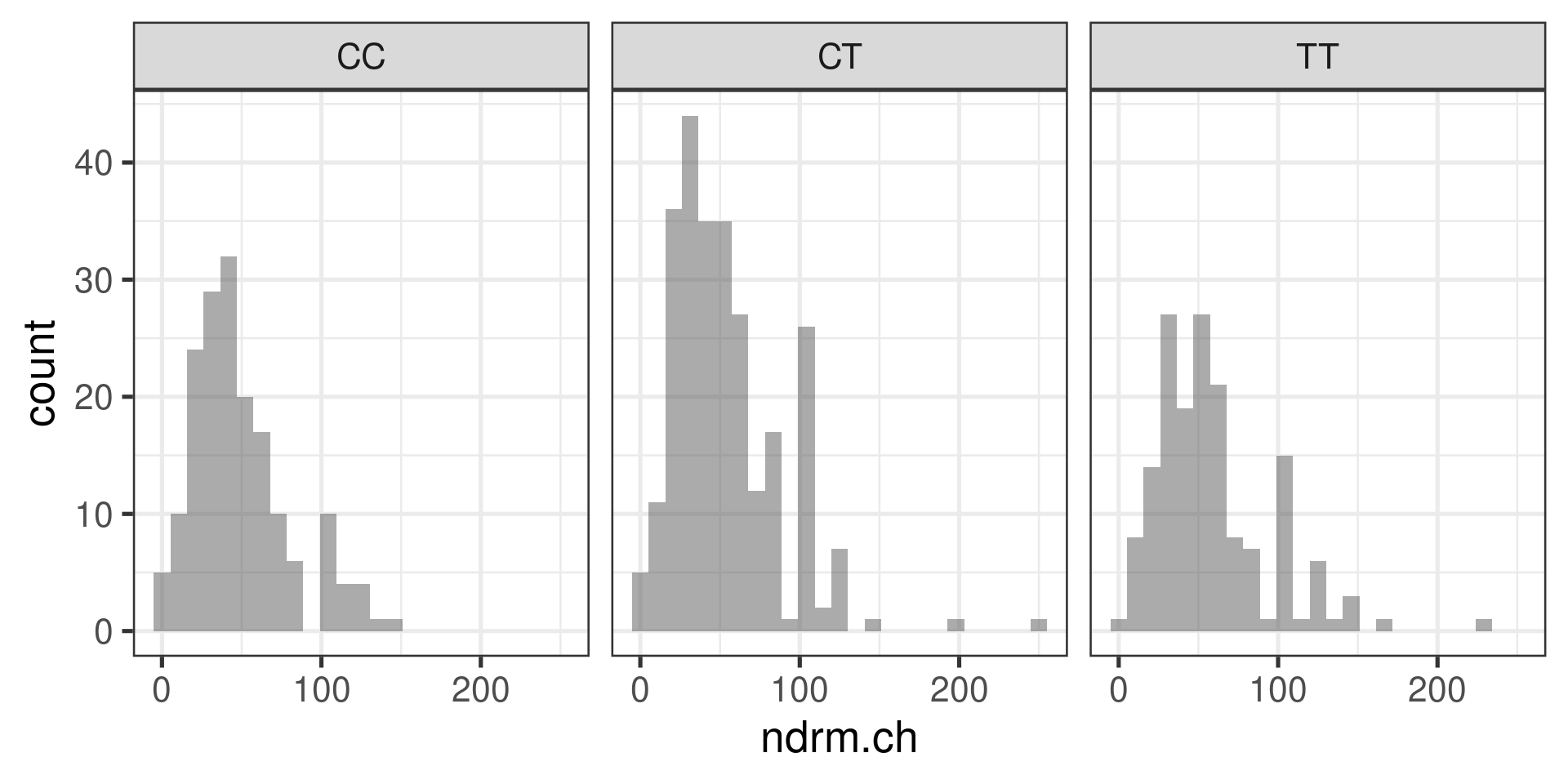

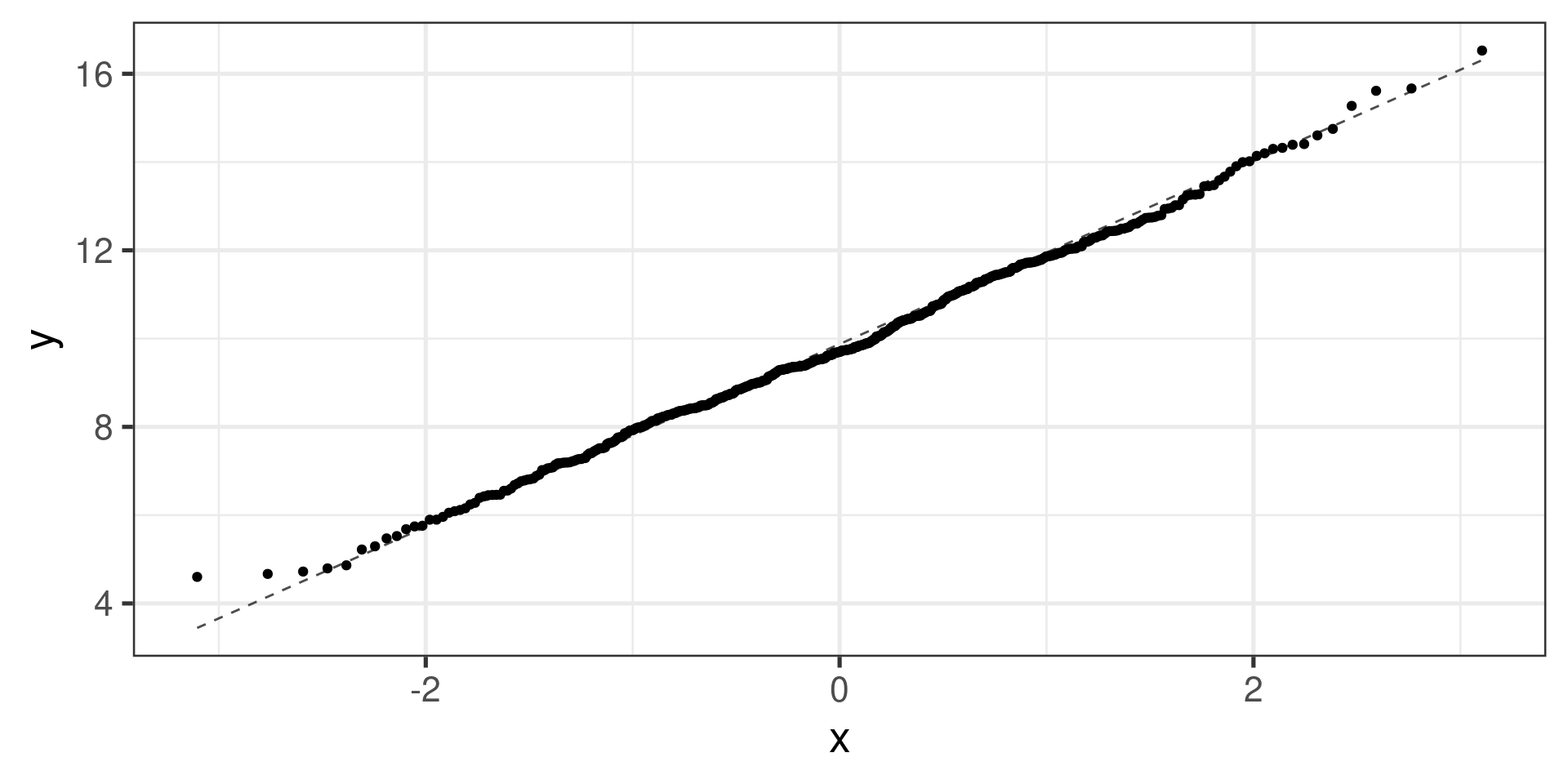
Normal probability plots (Q-Q plots)

gf_qq(~ndrm.ch | actn3.r577x,  data = famuss) |>
    gf_qqline()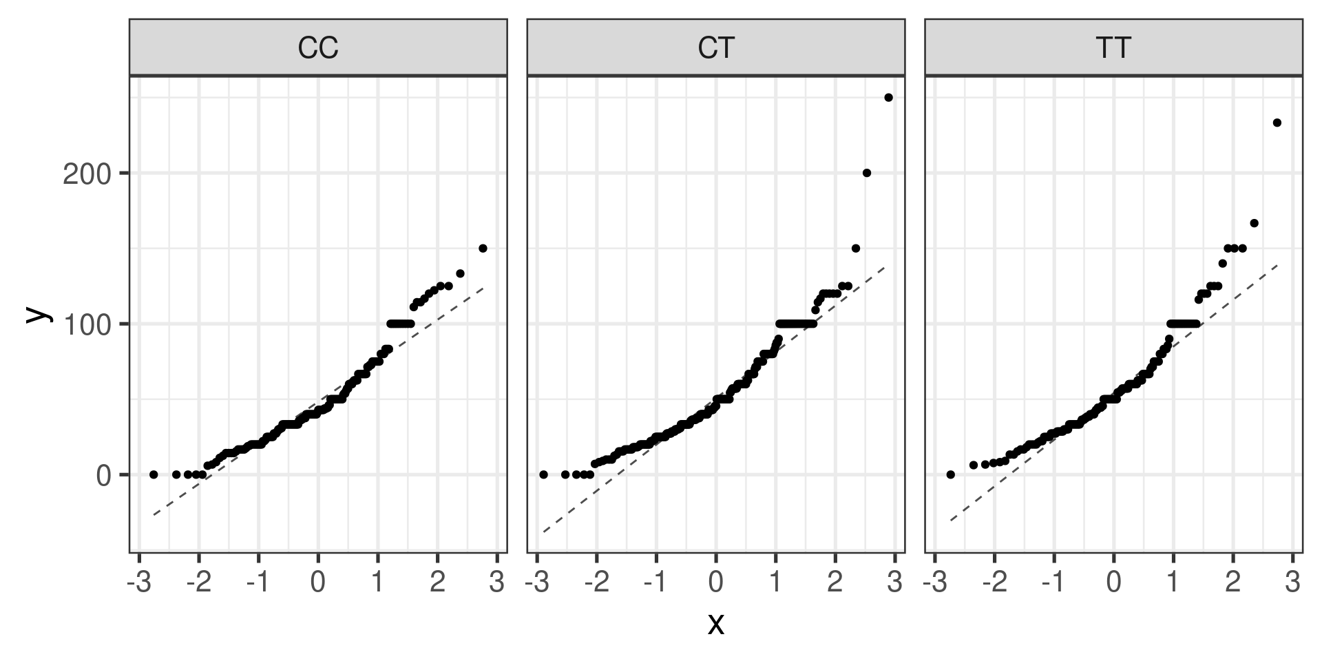

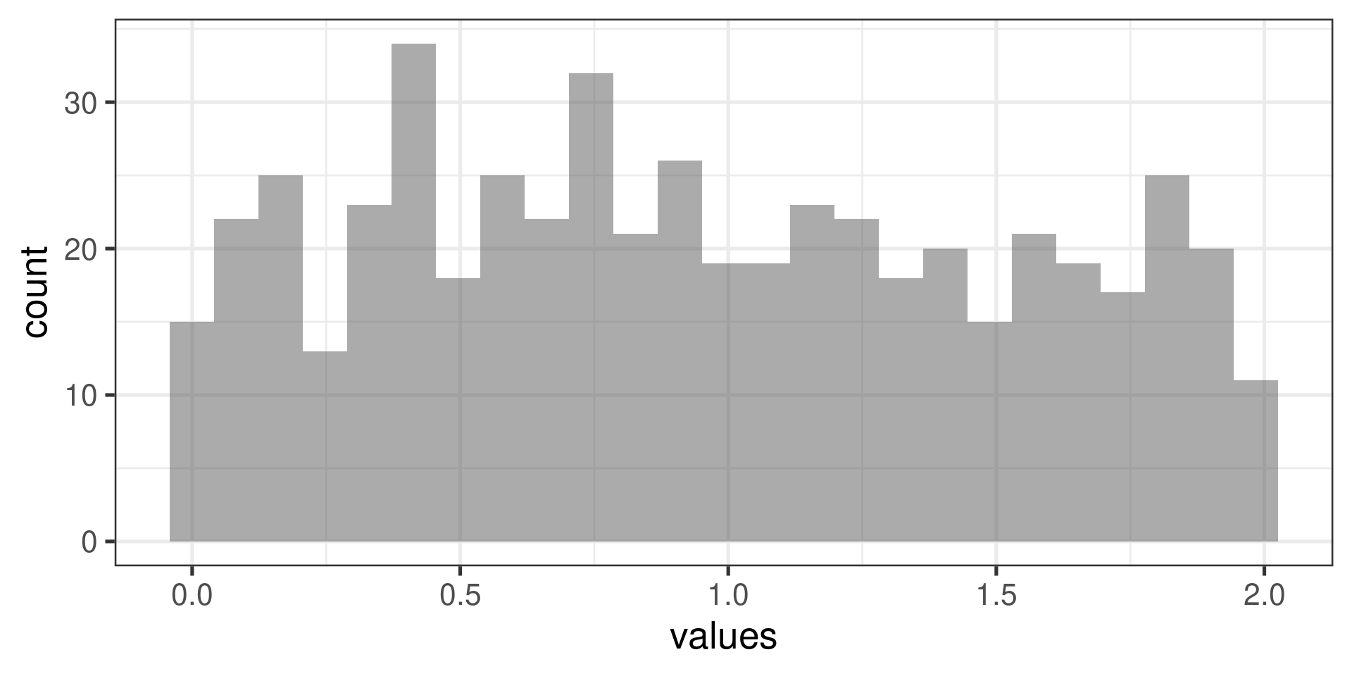
Normal probability plots examples

Right skewed distribution:

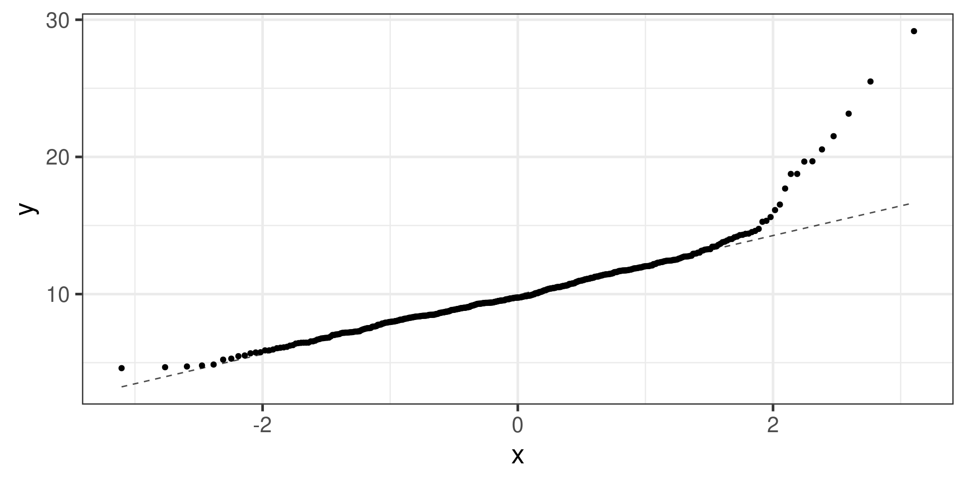
Normal probability plots examples

“Uniform” distribution:

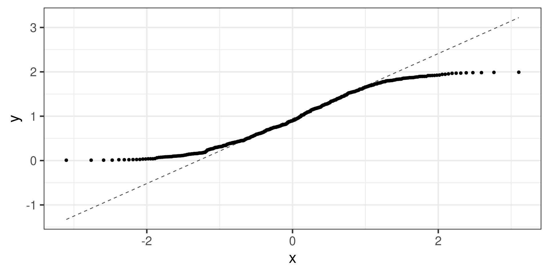
Normal probability plots examples

Normal distribution:

What next? (Pairwise comparisons)

If the $F$-test indicates that the group means are not all equal:

Proceed with pairwise comparisons to identify which group means are different.
Pairwise comparisons are made using the two-sample $t$-test for independent groups.

Problem: with multiple tests, the probability of type I error increases!

Type 1 error review

Hypothesis testing was originally intended for use in controlled experiments or studies with a small number of comparisons, such as ANOVA.

Recall that making a Type I error (rejecting $H_0$ when $H_0$ is true) theoretically occurs with probability $\alpha$.

Type I error rate is controlled by rejecting only when the $p$-value of a test is smaller than $\alpha$.
$\alpha$ is typically kept low.
With a single two-group comparison at $\alpha = 0.05$, there is a 5% chance of incorrectly identifying an association where none actually exists.

What about many tests?

What happens to Type I error when making several comparisons?

When conducting more than one $t$-test in an analysis…

The significance level ($\alpha$) used in each test controls the error rate for that test.
The experiment-wise error rate is the chance that at least one test will incorrectly reject $H_0$ when all tested null hypotheses are true.

The more tests we do, the higher the experiment-wise error rate gets!

Experiment-wise error rate

Suppose a scientist is using two $t$-tests to examine the possible association of each of two genes with a disease type. Assume the tests are independent and each are conducted at the $\alpha = 0.05$ significance level.

Let $A$ be the event of making a Type I error on the first test, and $B$ be the event of making a Type I error on the second test.

\[P(A) = P(B) = 0.05\]

The probability of making at least one error is equal to the complement of the event that a Type I error is not made with either test.

\[1 - \left[P\left(A^C\right) P\left(B^C\right) \right] = 1 - (1 - 0.05)^2 = 0.0975\]

Thus, when making two independent $t$-tests, there is about a 10% chance of making at least one Type I error; the experiment-wise error rate is 10%.

Experiment-wise error rate

With 10 tests… \[\text{experiment-wise error rate}= 1 - (1 - 0.05)^{10} = 0.401\]

With 25 tests… \[\text{experiment-wise error rate}= 1 - (1 - 0.05)^{25} = 0.723\]

With 100 tests… \[\text{experiment-wise error rate}= 1 - (1 - 0.05)^{100} = 0.994\]

With 100 independent tests, there is a 99.4% chance an investigator will make at least one Type I error!

Bonferroni correction

To maintain the overall Type I error rate at $\alpha$, each pairwise comparison is conducted at an adjusted significance level denoted $\alpha^\star$.
The Bonferroni correction is one method for adjusting $\alpha$. \[\alpha^\star = \alpha/K, \text{ where } K = \text{ the number of tests}\] \[K = \binom{k}{2} = \frac{k(k-1)}{2} \text{ for $k$ groups}\]
Bonferroni correction is a very stringent (i.e., conservative) correction, made under the assumption that all tests are independent.

Pairwise comparisons …

  actn3.r577x min   Q1 median   Q3   max     mean       sd   n missing
1          CC   0 30.0   42.9 66.7 150.0 48.89422 29.95608 173       0
2          CT   0 30.0   45.5 71.4 250.0 53.24904 33.23148 261       0
3          TT   0 33.3   50.0 75.0 233.3 58.08385 35.69133 161       0

$H_0: \mu_{\text{CC}} = \mu_{\text{CT}}$
$H_0: \mu_{\text{CC}} = \mu_{\text{TT}}$
$H_0: \mu_{\text{CT}} = \mu_{\text{TT}}$

$\alpha^\star = \frac{\alpha}{3} = \frac{0.05}{3} \approx 0.0167$

CC vs. CT

  actn3.r577x min   Q1 median   Q3   max     mean       sd   n missing
1          CC   0 30.0   42.9 66.7 150.0 48.89422 29.95608 173       0
2          CT   0 30.0   45.5 71.4 250.0 53.24904 33.23148 261       0
3          TT   0 33.3   50.0 75.0 233.3 58.08385 35.69133 161       0

$\displaystyle SE = \sqrt{\frac{s_\text{CC}^2}{n_\text{CC}} + \frac{s_\text{CT}^2}{n_\text{CT}}} = \sqrt{\frac{29.96^2}{173} + \frac{33.23^2}{261}} = 3.069$
$\displaystyle t = \frac{\overline{X}_\text{CC} - \overline{X}_\text{CT}}{SE} = \frac{48.89 - 53.25}{3.069} = -1.421$
which gives the $p$-value of $0.1572366$.
Compare to $\alpha^\star \approx 0.0167$

CT vs. TT

  actn3.r577x min   Q1 median   Q3   max     mean       sd   n missing
1          CC   0 30.0   42.9 66.7 150.0 48.89422 29.95608 173       0
2          CT   0 30.0   45.5 71.4 250.0 53.24904 33.23148 261       0
3          TT   0 33.3   50.0 75.0 233.3 58.08385 35.69133 161       0

$\displaystyle SE = \sqrt{\frac{s_\text{CT}^2}{n_\text{CT}} + \frac{s_\text{TT}^2}{n_\text{TT}}} = \sqrt{\frac{33.23^2}{261} + \frac{35.69^2}{161}} = 3.485$
$\displaystyle t = \frac{\overline{X}_\text{CC} - \overline{X}_\text{CT}}{SE} = \frac{53.24 - 58.08}{3.485} = -1.389$
which gives the $p$-value of $0.1667724$.
Compare to $\alpha^\star \approx 0.0167$

CC vs. TT

  actn3.r577x min   Q1 median   Q3   max     mean       sd   n missing
1          CC   0 30.0   42.9 66.7 150.0 48.89422 29.95608 173       0
2          CT   0 30.0   45.5 71.4 250.0 53.24904 33.23148 261       0
3          TT   0 33.3   50.0 75.0 233.3 58.08385 35.69133 161       0

$\displaystyle SE = \sqrt{\frac{s_\text{CC}^2}{n_\text{CC}} + \frac{s_\text{TT}^2}{n_\text{TT}}} = \sqrt{\frac{29.96^2}{173} + \frac{35.69^2}{161}} = 3.619$
$\displaystyle t = \frac{\overline{X}_\text{CC} - \overline{X}_\text{CT}}{SE} = \frac{48.89 - 58.08}{3.619} = -2.539$
which gives the $p$-value of $0.0120682$.
Compare to $\alpha^\star \approx 0.0167$

Pairwise comparisons …

with(famuss, pairwise.t.test(ndrm.ch, actn3.r577x, p.adj = "none"))


    Pairwise comparisons using t tests with pooled SD 

data:  ndrm.ch and actn3.r577x 

   CC    CT   
CT 0.179 -    
TT 0.011 0.144

P value adjustment method: none

Comparing p-values to $\alpha = 0.05/K$ where $K = 3$.

Pairwise comparisons …

with(famuss, pairwise.t.test(ndrm.ch, actn3.r577x, p.adj = "bonf"))


    Pairwise comparisons using t tests with pooled SD 

data:  ndrm.ch and actn3.r577x 

   CC    CT   
CT 0.537 -    
TT 0.034 0.433

P value adjustment method: bonferroni

Comparing p-values to $\alpha = 0.05$ (they are already adjusted).

Math 132B

FAMuSS Study

FAMuSS Study

We had multiple groups

FAMuSS Example

Or, what we did

Or, what we did

Simulated null distribution

Simulated null distribution

The \(p\)-value

Letting R do all the work

Assumptions for ANOVA

Boxplots

Histograms

Normal probability plots (Q-Q plots)

Normal probability plots examples

Normal probability plots examples

Normal probability plots examples

What next? (Pairwise comparisons)

Type 1 error review

What about many tests?

Experiment-wise error rate

Experiment-wise error rate

Bonferroni correction

Pairwise comparisons …

CC vs. CT

CT vs. TT

CC vs. TT

Pairwise comparisons …

Pairwise comparisons …