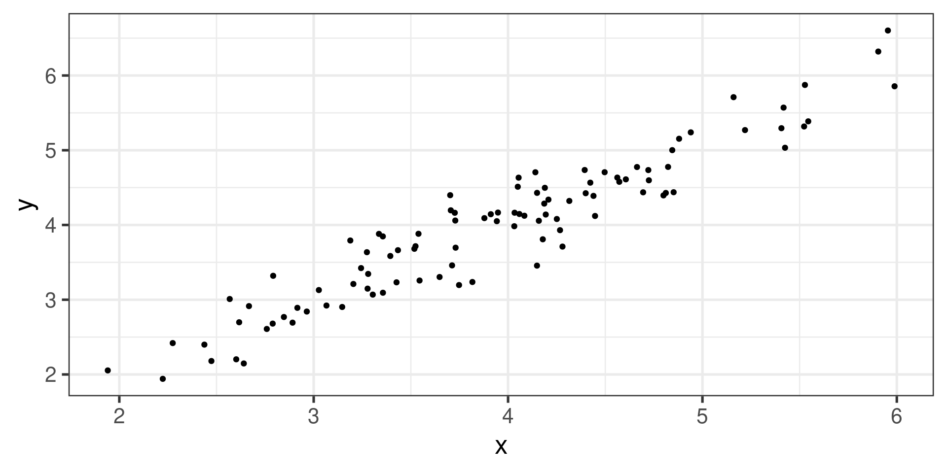
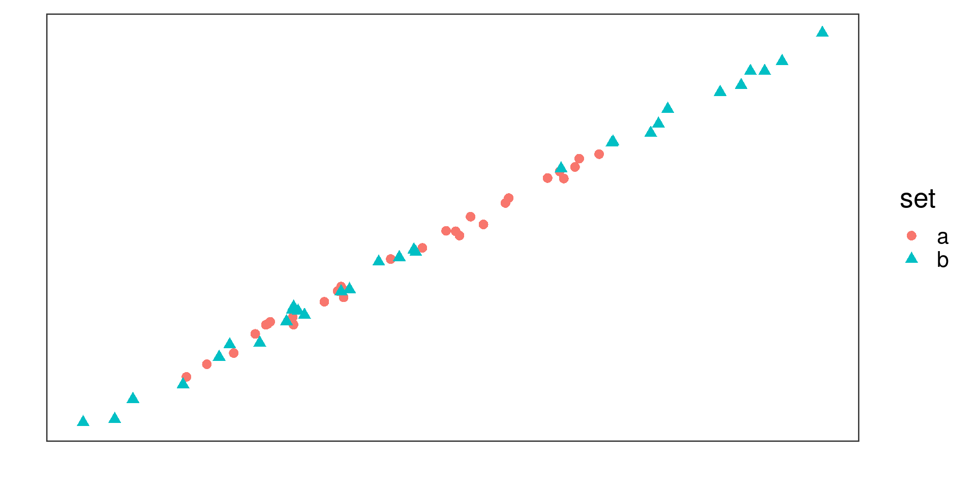
Example 1
![]()
Positive linear association
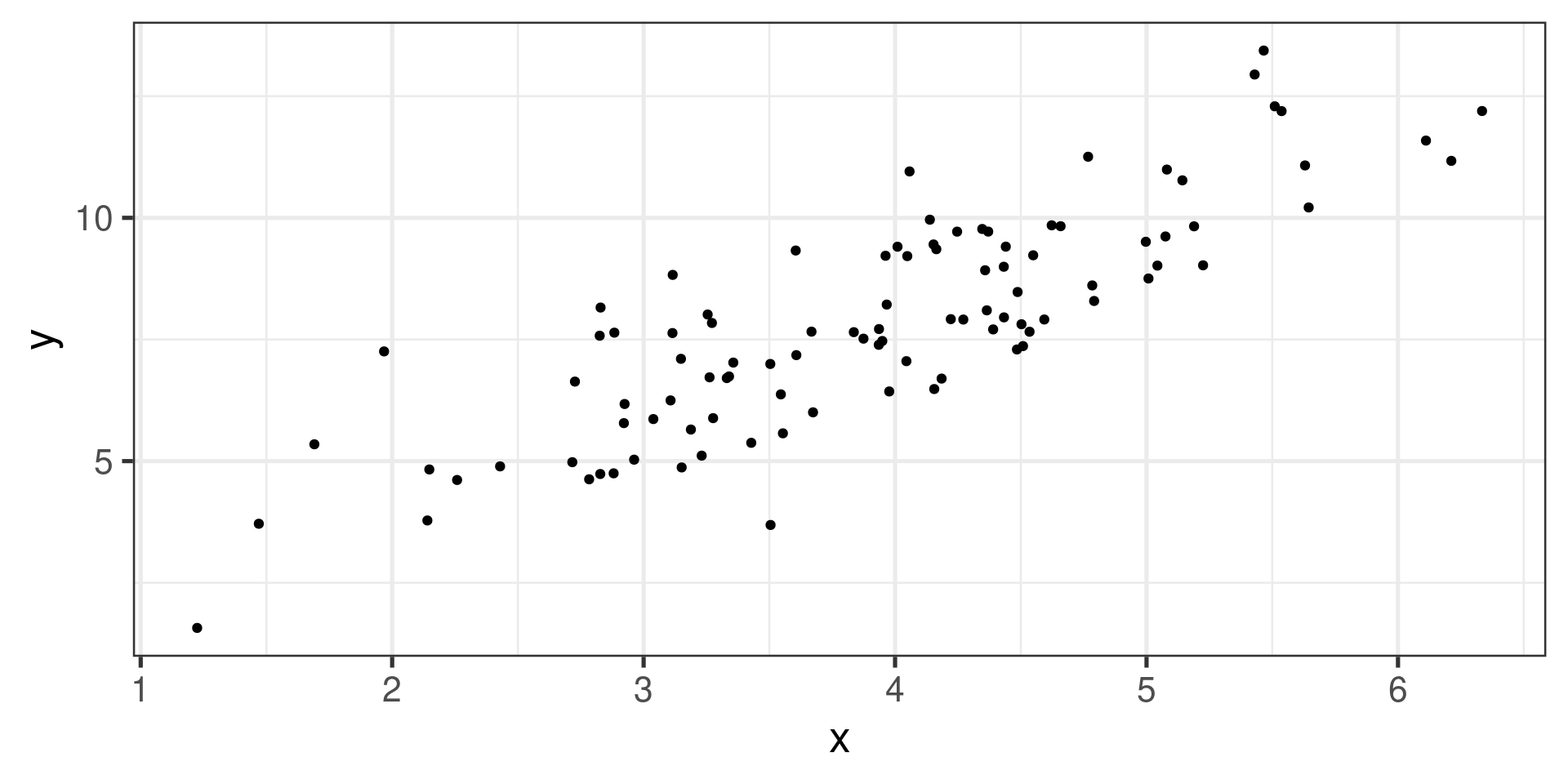
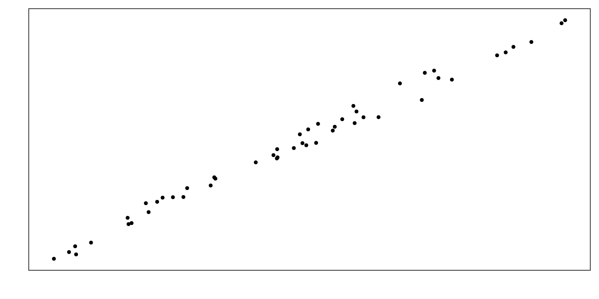
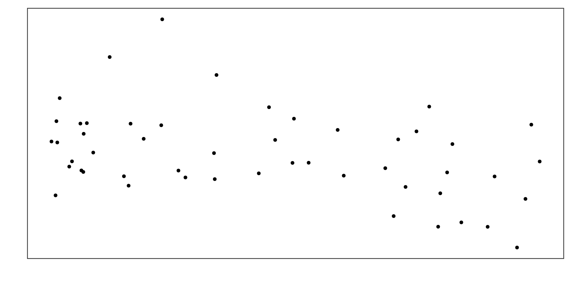
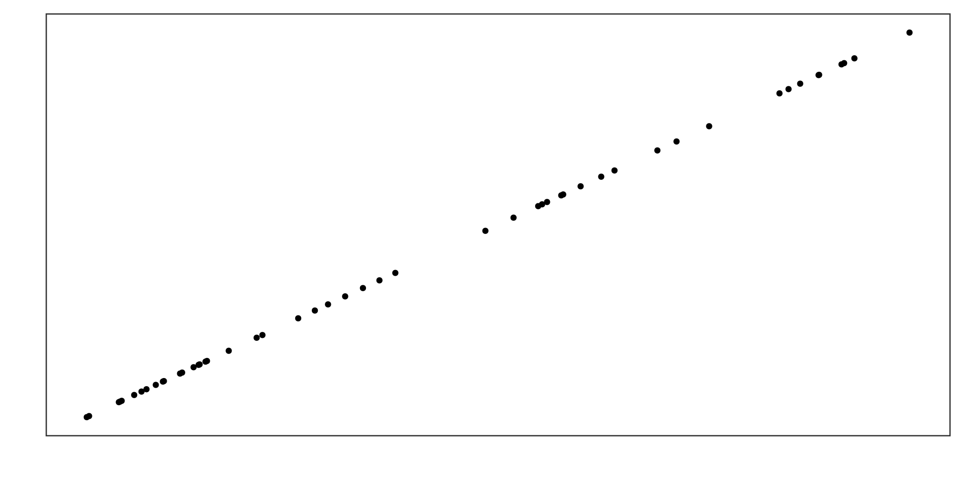
Example 2
![]()
Positive linear association, much weaker
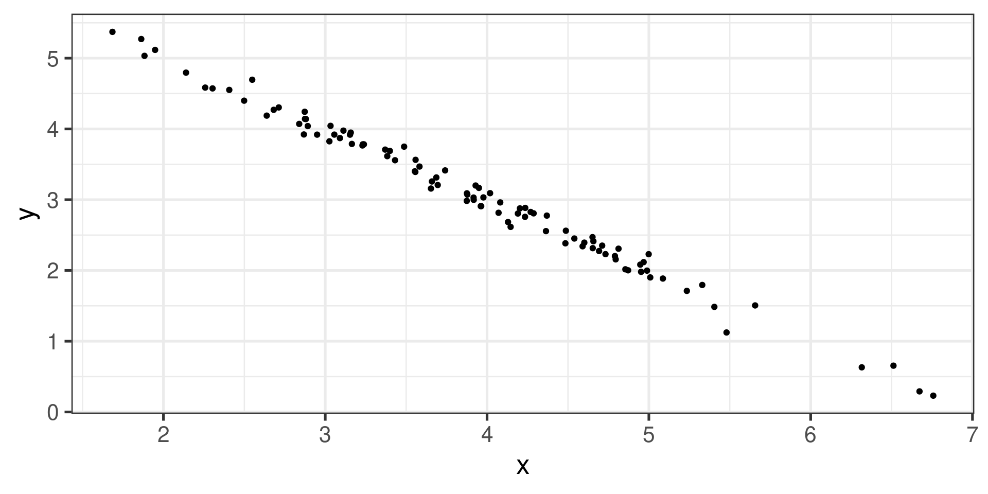
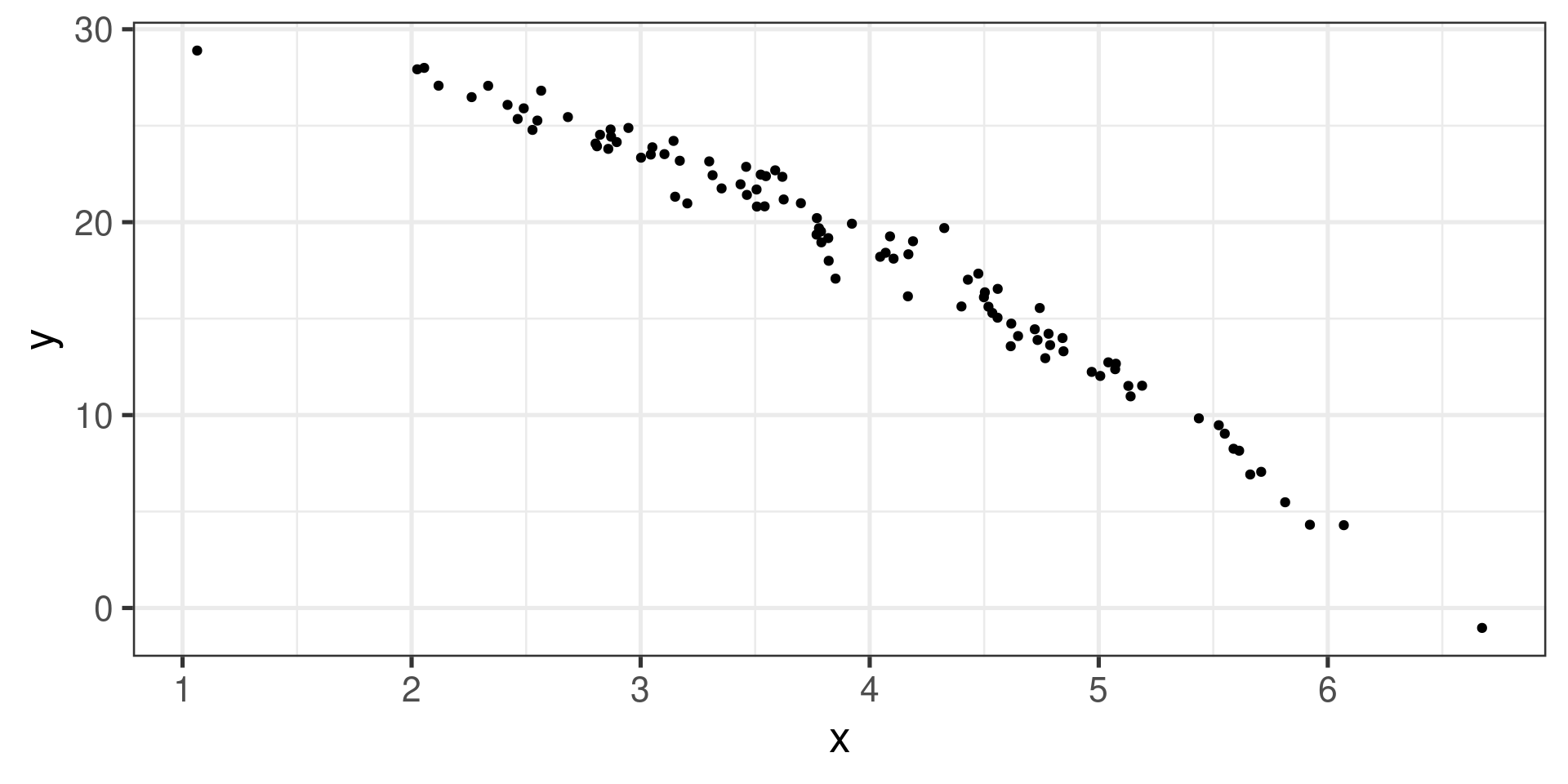
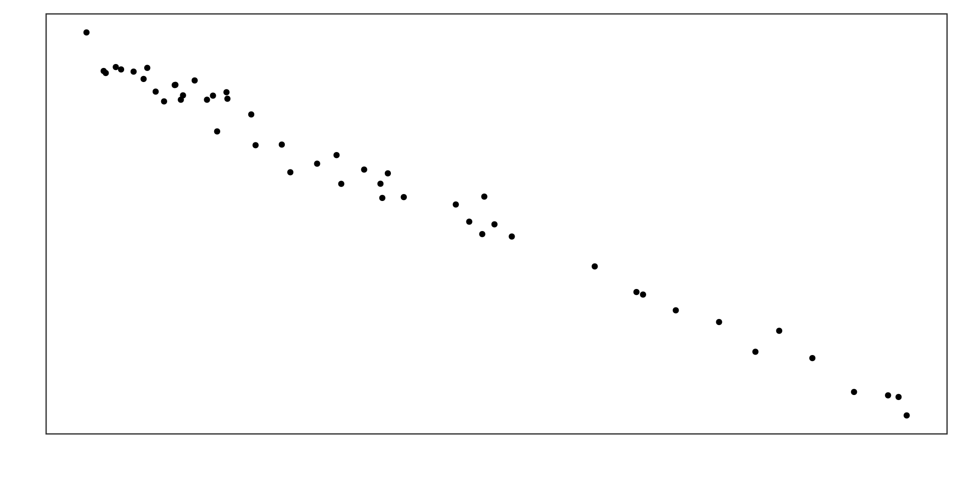
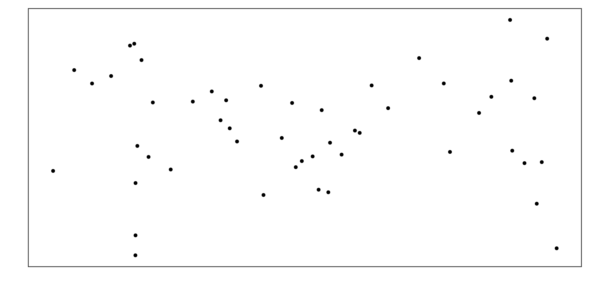
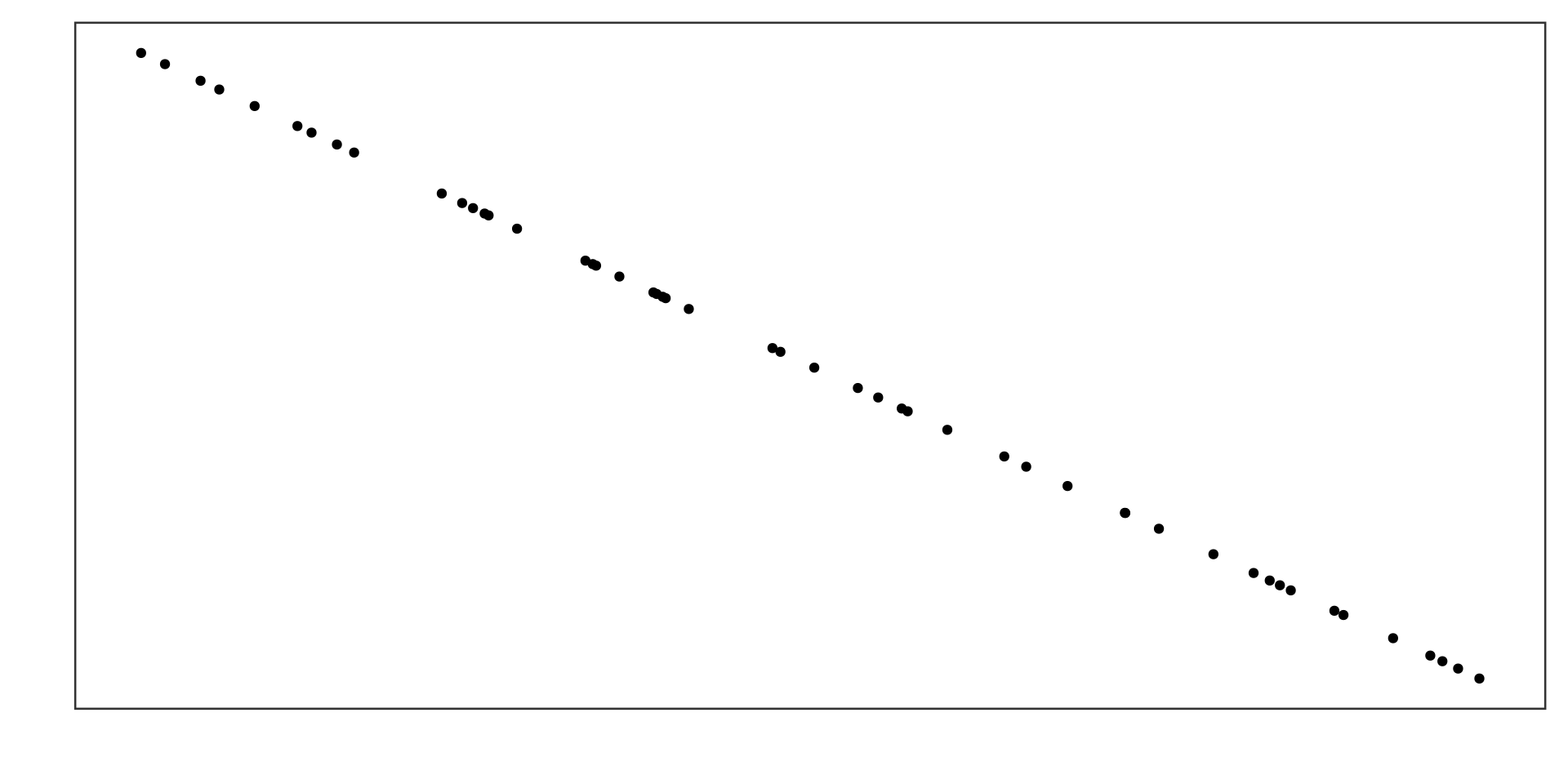
Example 3
![]()
Strong negative linear association
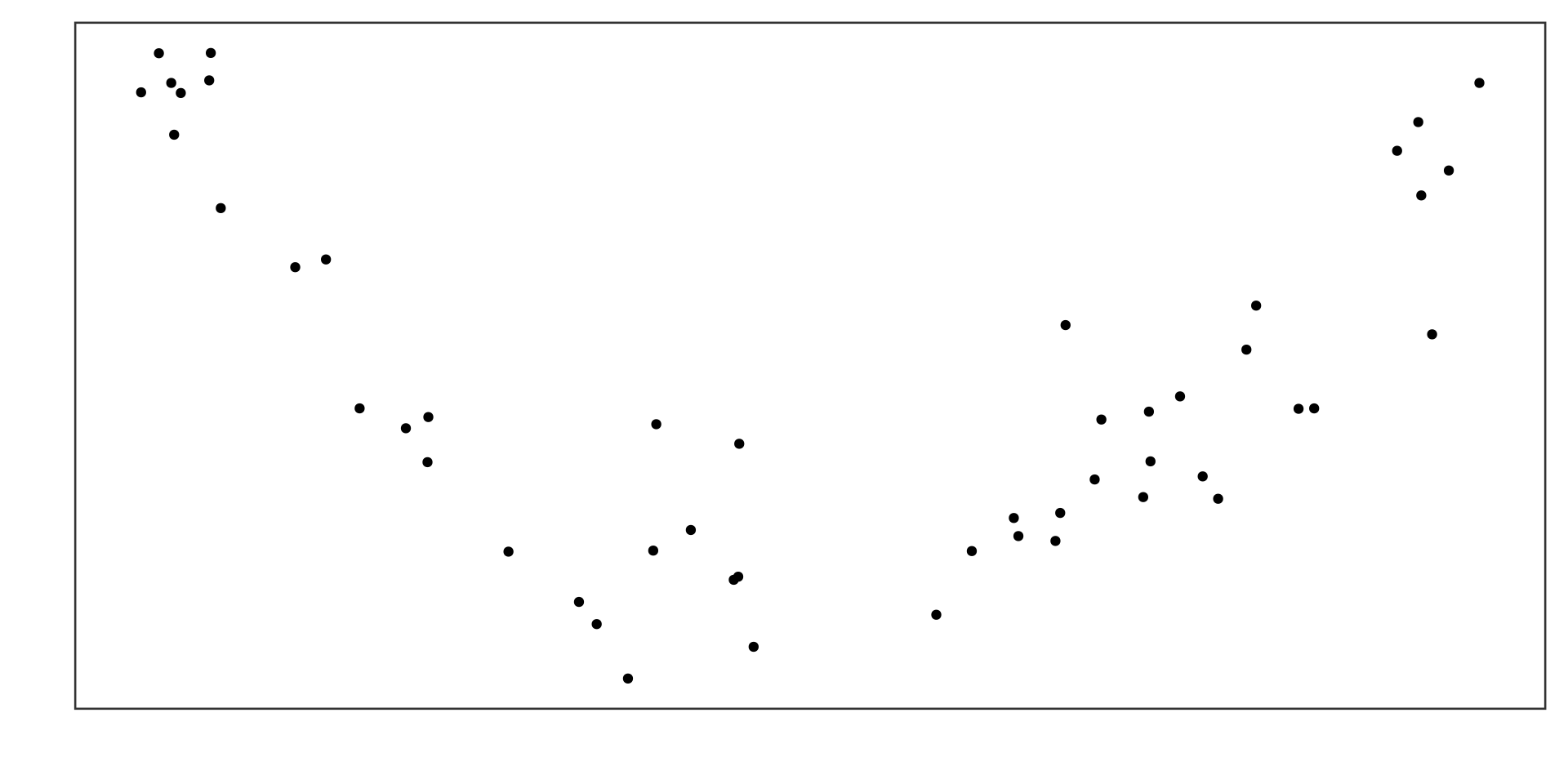
Example 4
![]()
Non-linear association
Example 5
![]()
Non-linear association
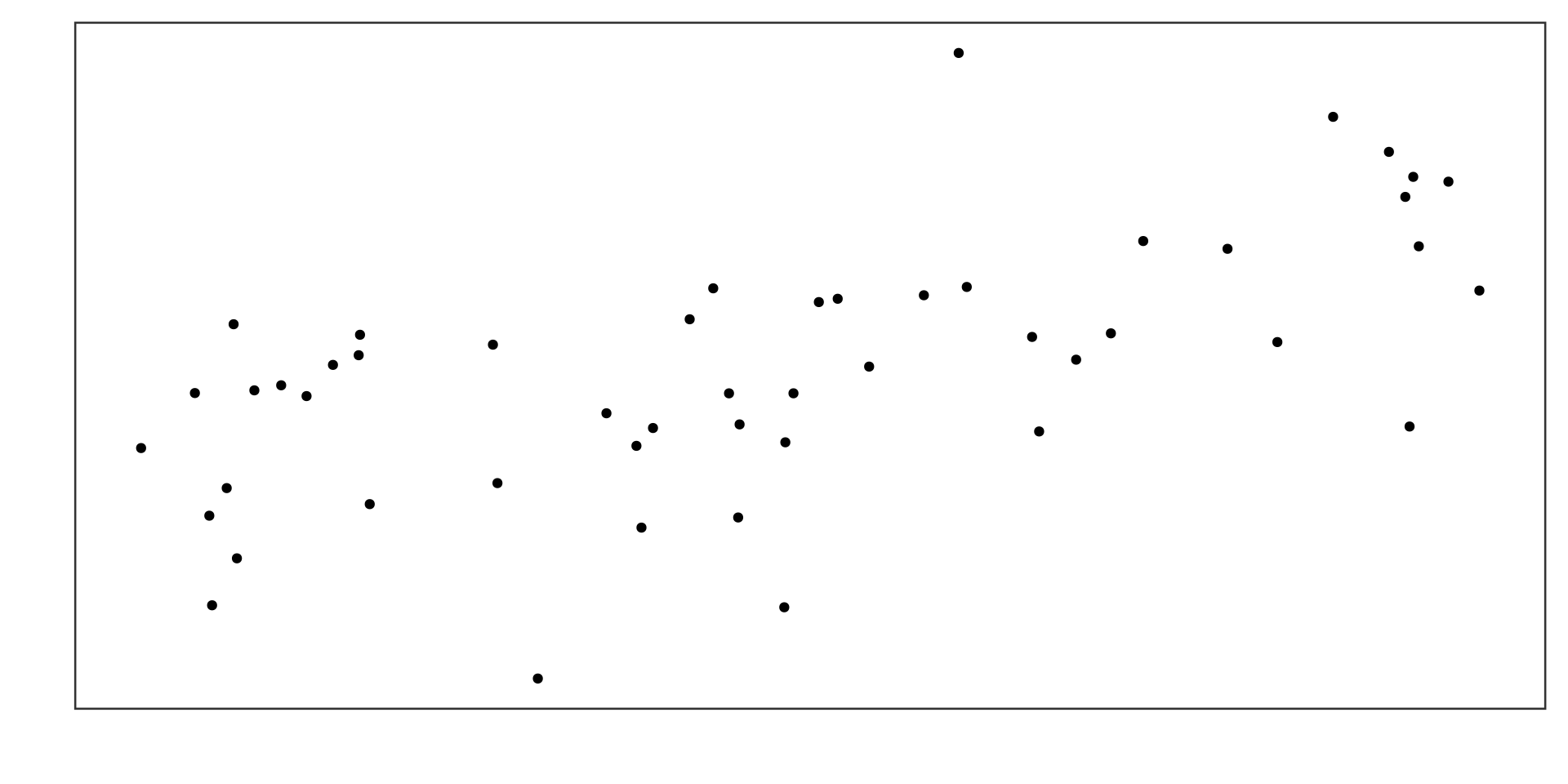
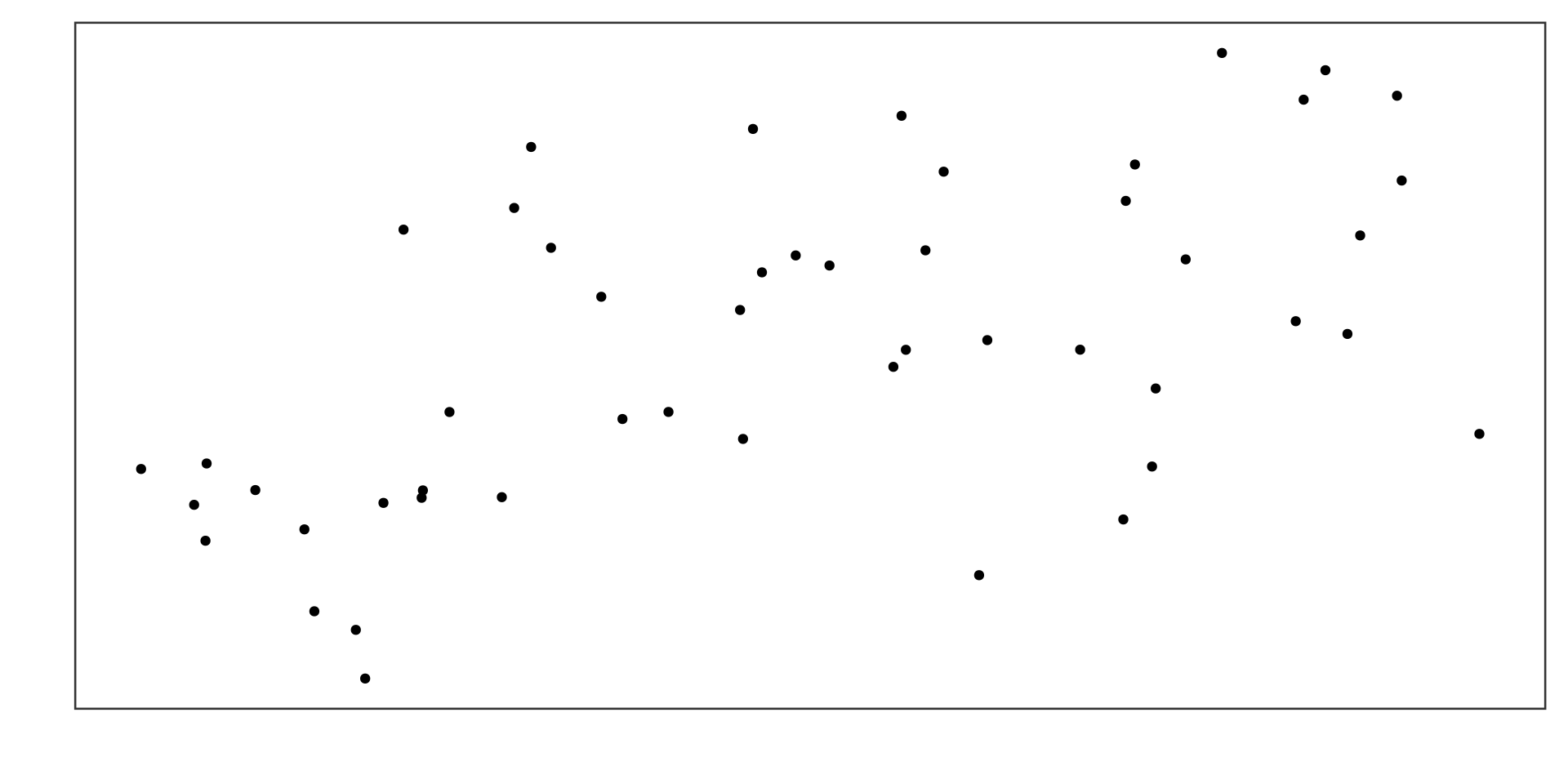
Example 6
![]()
Unclear (very weak linear) association
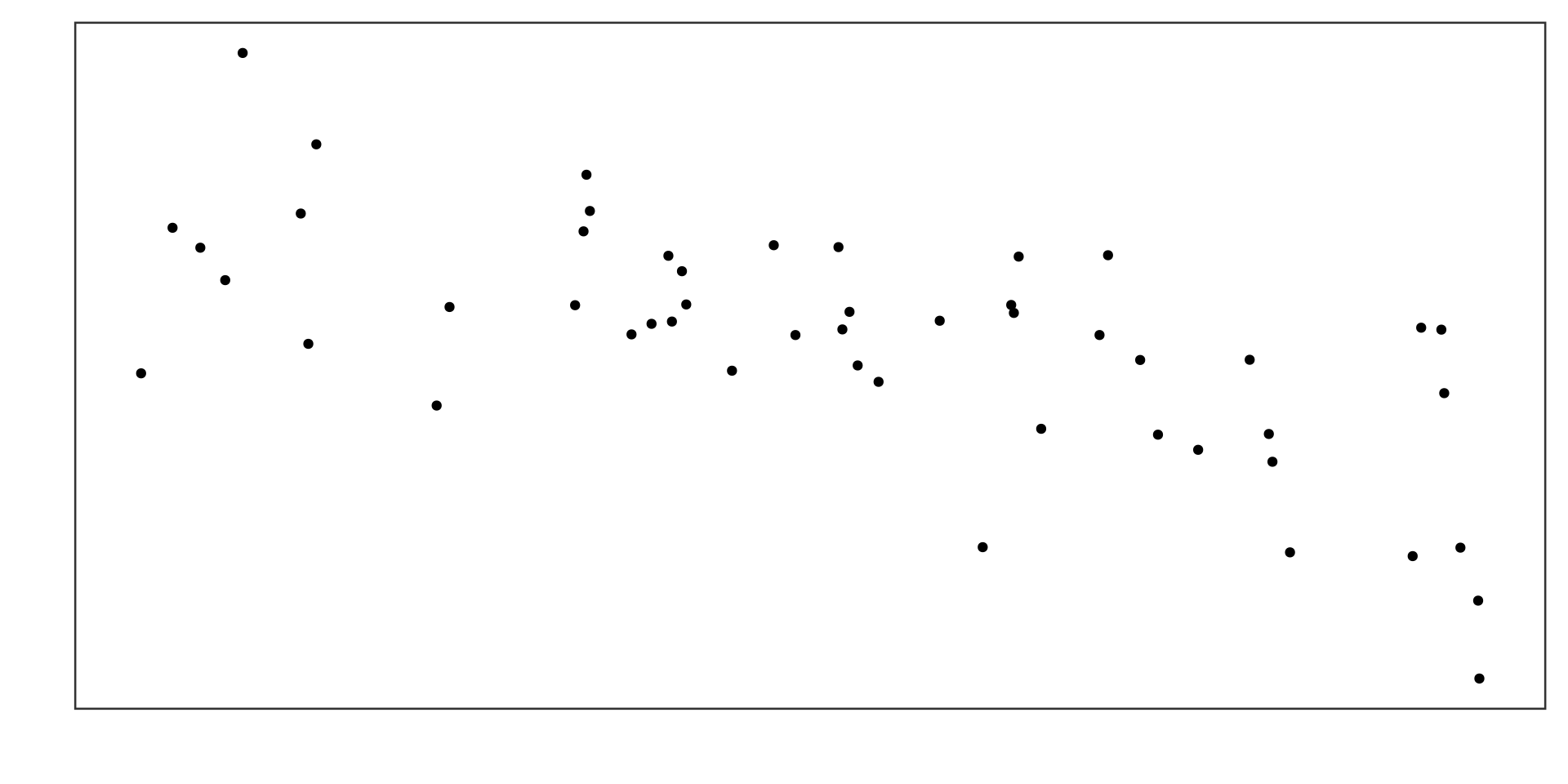
Example 7
![]()
No association, or very weak association
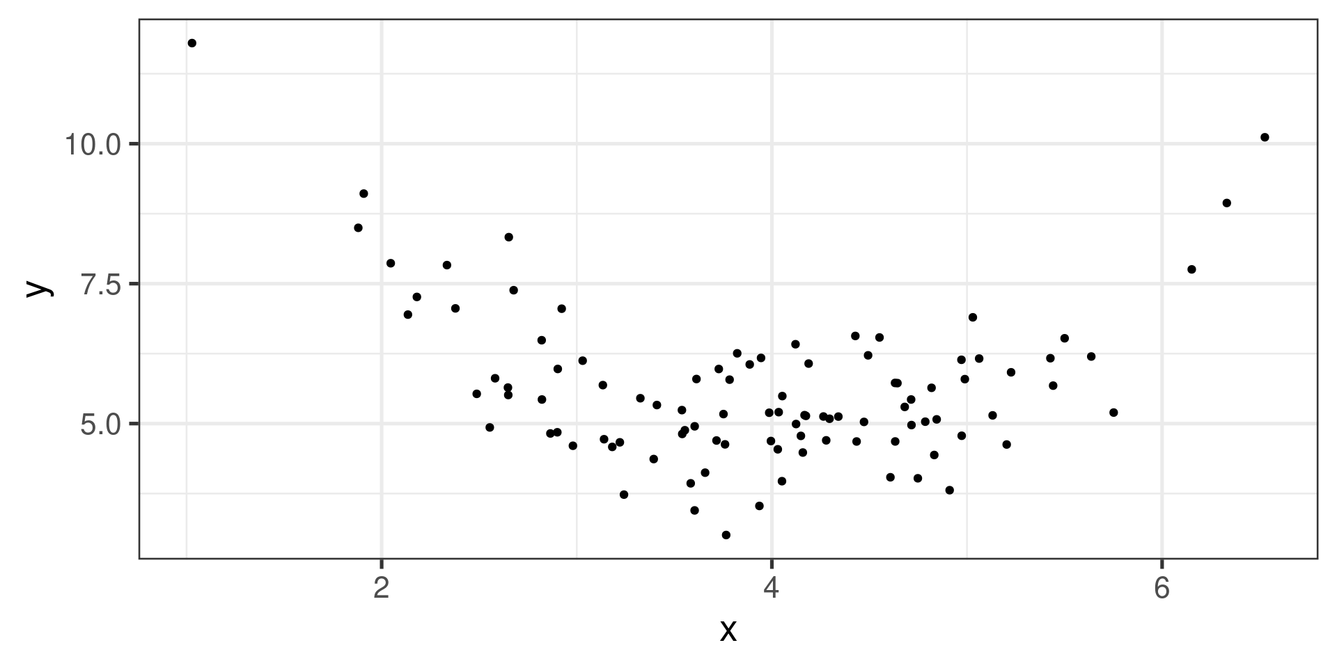
Strength of Linear association
![]()
\(\overline{x} = 4.0508382\), \(\overline{y} = 7.9387814\)
Not quite there yet
![]()
Mean of \((x- \overline{x})(y - \overline{y})\):
How to fix this problem?
Trying to use the mean of \((x - \overline{x})(y - \overline{y})\) to measure strength of correlation.
Two data sets with similar amount of “scatter” give us very different results: the data set with larger spread has larger deviations.
How do we measure spread?
\[\text{Mean of } \frac{x - \overline{x}}{s_x} \frac{y - \overline{y}}{s_y}\]
Almost there
![]()
Mean of \(\frac{x- \overline{x}}{s_x}\frac{y - \overline{y}}{s_y}\):
Last (optional) adjustment
-
Mean of \(\frac{x- \overline{x}}{s_x}\frac{y - \overline{y}}{s_y}\):
\[\frac{1}{n}\sum\frac{x- \overline{x}}{s_x}\frac{y - \overline{y}}{s_y}\]
-
Small change to improve estimate properties:
\[\frac{1}{\color{red}{n-1}}\sum\frac{x- \overline{x}}{s_x}\frac{y - \overline{y}}{s_y}\]
Correlation coefficient \(r\)
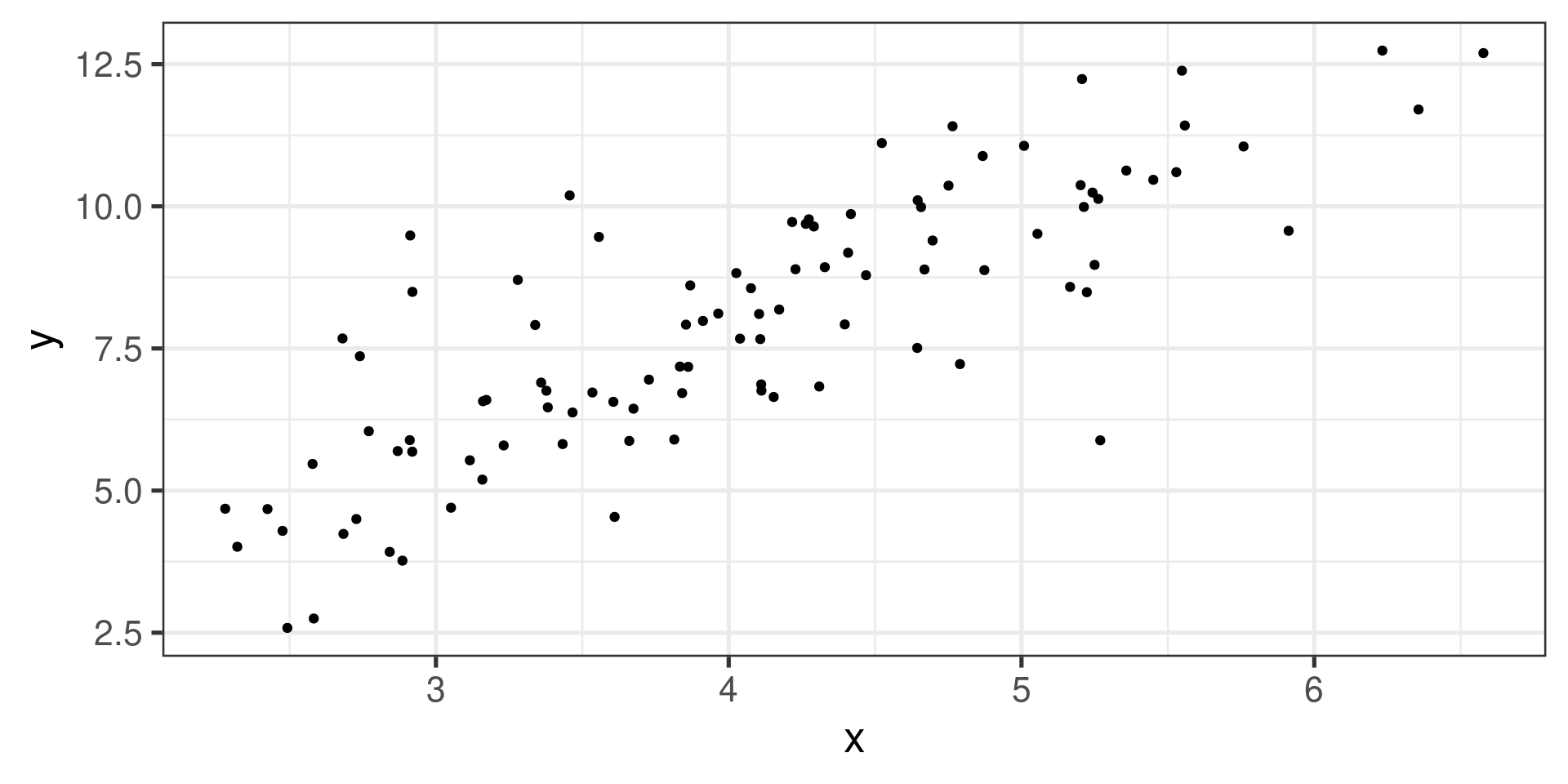
Strong positive correlation
![]()
\(r = 0.995\)
Strong negative correlation
![]()
\(r = -0.993\)
Weak positive correlation
![]()
\(r = 0.611\)
Weak negative correlation
![]()
\(r = -0.672\)
Very weak positive correlation
![]()
\(r = 0.561\)
Very weak negative correlation
![]()
\(r = -0.391\)
No association
![]()
\(r = 0.003\)
Nonlinear association
![]()
Correlation coefficient not useful!
Perfect positive correlation
![]()
\(r = 1\)
Perfect negative correlation
![]()
\(r = -1\)
Strength of Linear association
Not applicable if the scatterplot shows a nonlinear association!
Use only if scatterplot shows a linear association or no clear association
Start by moving data so that the point \((0,0)\) is in the center (subtracting means): \(x - \overline{x}\) and \(y - \overline{y}\).
Multiply together and calculate the “mean”
To compensate for different spreads, divide by both standard deviations
Pearson’s correlation coefficient
\[r = \frac{\text{mean}((x - \overline{x})\cdot (y - \overline{y}))}{\sigma_x\cdot\sigma_y}\]
where:
-
\(\overline{x}\) is the sample mean of the \(x\) variable
-
\(\overline{y}\) is the sample mean of the \(y\) variable
-
\(\sigma_x\) is the sample standard deviation of the \(x\) variable
-
\(\sigma_y\) is the sample standard deviation of the \(y\) variable
In R: cor(x,y) or cor(y ~ x, data = ...)
Properties:
Between \(-1\) and \(1\)
\(r > 0\) indicate positive correlation
\(r < 0\) indicates negative correlation
if \(\left\lvert r\right\rvert\) is larger, it means stronger correlation
Hypothesis testing
Population correlation coefficient is denoted \(\rho\) (rho).
\(H_0\): There is no correlation (\(\rho = 0\)).
\(H_A\): There is a (positive, negative) correlation (\(\rho \neq (>, <) 0\)).
We have a sample with correlation coefficient \(r\), we want to know if it is a strong enough evidence to reject \(H_0\).
T-test for correlation
We can also calculate a t-statistic:
\[t = r\sqrt{\frac{n-2}{1-r^2}}\]
This has t-distribution with \(n-2\) degrees of freedom.
OK, so there is a linear association
What now?
Find a mathematical model for the association:
\[y = ax + b\]
Data is scattered, so the relation will actually be
\[ y = ax + b + \text{ "noise"} \]
Terminology
predicted value of \(y\): \[\widehat{y} = ax + b\]
actual or observed value of \(y\): \[y = \widehat{y} + e\]
\(e = y - \widehat{y}\) is the residual
“Ideal” model
- Residuals are as small as possible.
- The sum of squares of the residuals should be as small as possible.
- Line of best fit aka least squares line.
- Residuals are independent of \(x\).
-
No association between \(x\) and the residuals.
- The variation of the residuals should not depend on \(x\) (homoscedasticity)
Parameters vs. statistics again
The population model: \[\widehat{y} = \beta_0 + \beta_1 x\]
The estimate based on the sample: \[\widehat{y} = b_0 + b_1 x\]
\(\widehat{y}\) is the predicted value
\(b_0\) is the point estimate of \(\beta_0\): the intercept.
\(b_1\) is the point estimate of \(\beta_1\): the rate of change.
Version with the “noise”
The population model: \[y = \beta_0 + \beta_1 x + \varepsilon\]
The estimate based on the sample: \[y = b_0 + b_1 x + e\]
\(e\) is the residual (noise)
\(\varepsilon\) is the random variable representing the residuals
Calculating the point estimates
lm(RFFT ~ Age, data = prevend.samp)
Call:
lm(formula = RFFT ~ Age, data = prevend.samp)

Coefficients:
(Intercept)          Age
    137.550       -1.261
The least squares line can be written as \[
\widehat{\text{RFFT}} = 137.55 - 1.26 (\text{Age})
\]