
lm(RFFT ~ Age, data = prevend.samp)
Call:
lm(formula = RFFT ~ Age, data = prevend.samp)

Coefficients:
(Intercept)          Age
137.550 -1.261 Class 26
Two numerical variables
What kind of association is there between them?
Lots of possibilities
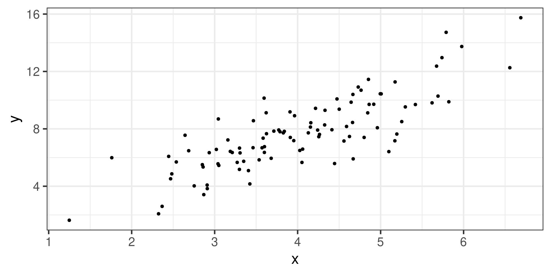
First resource: scatterplot!
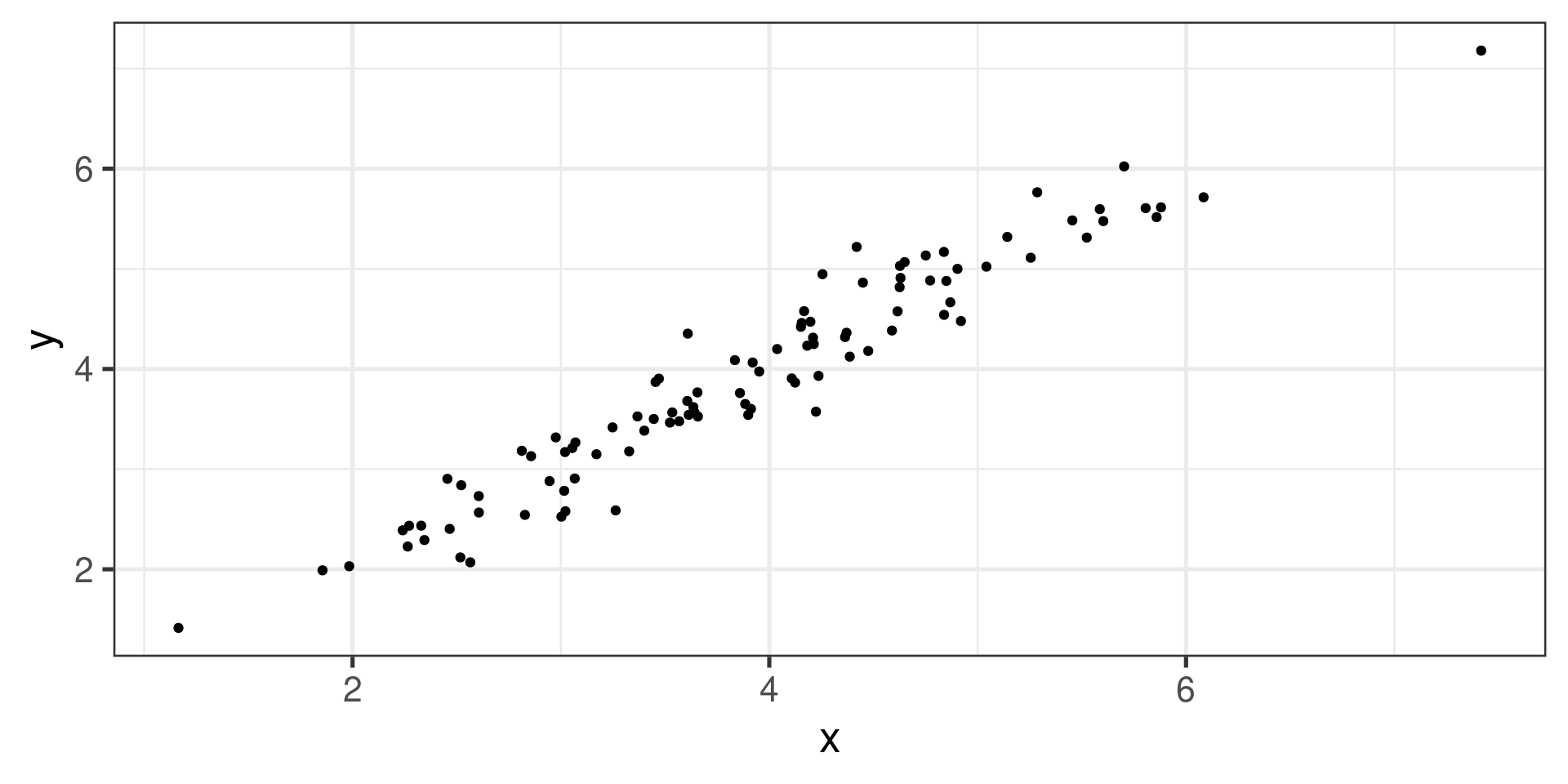
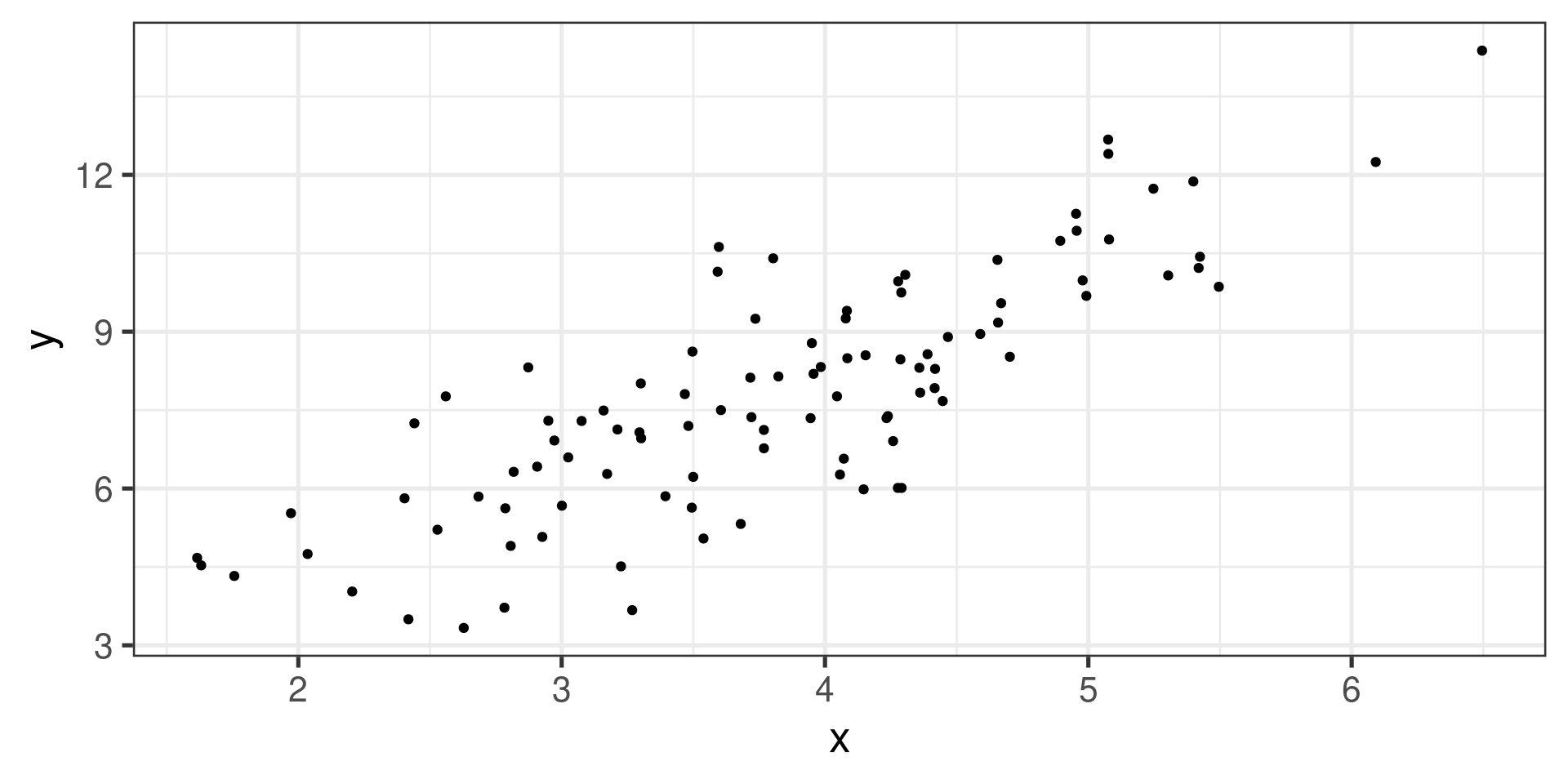
Positive linear association
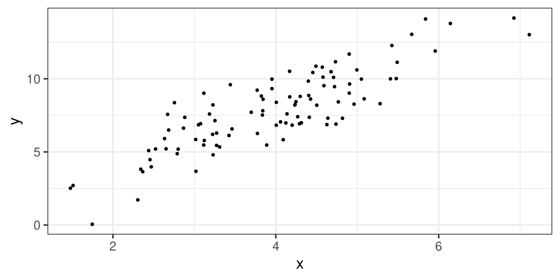
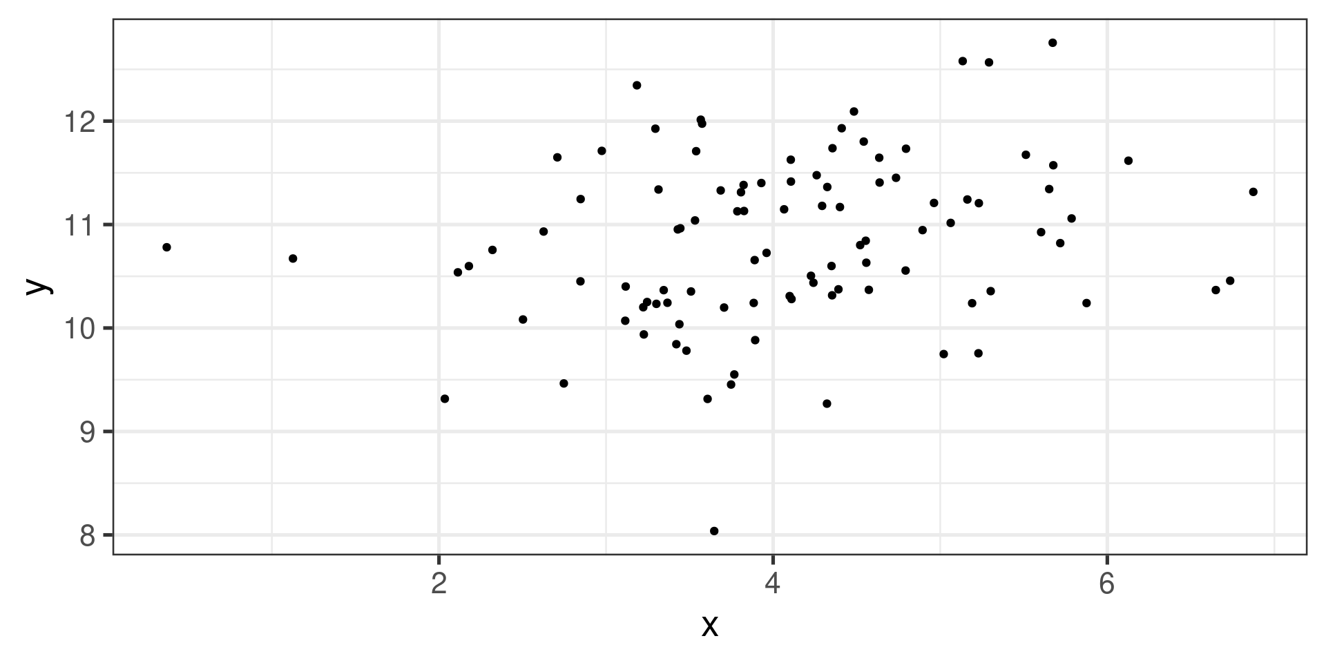
Positive linear association, much weaker
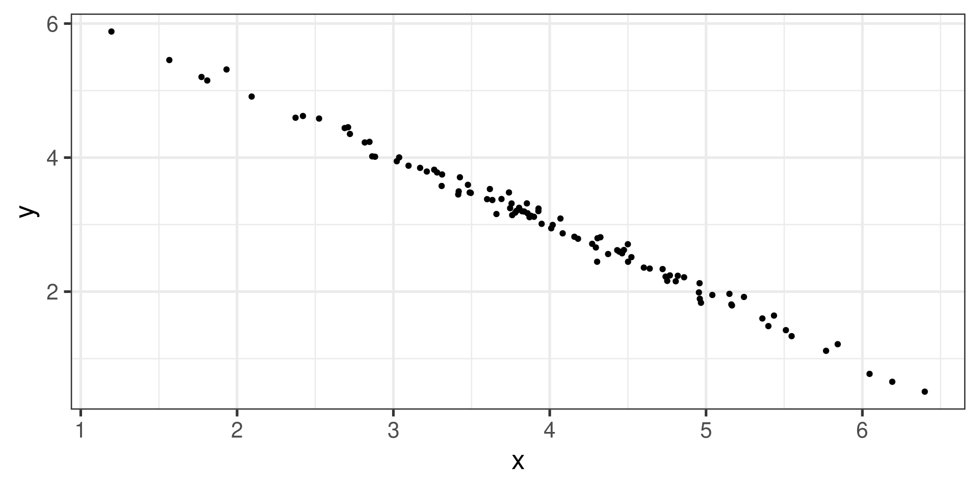
Strong negative linear association
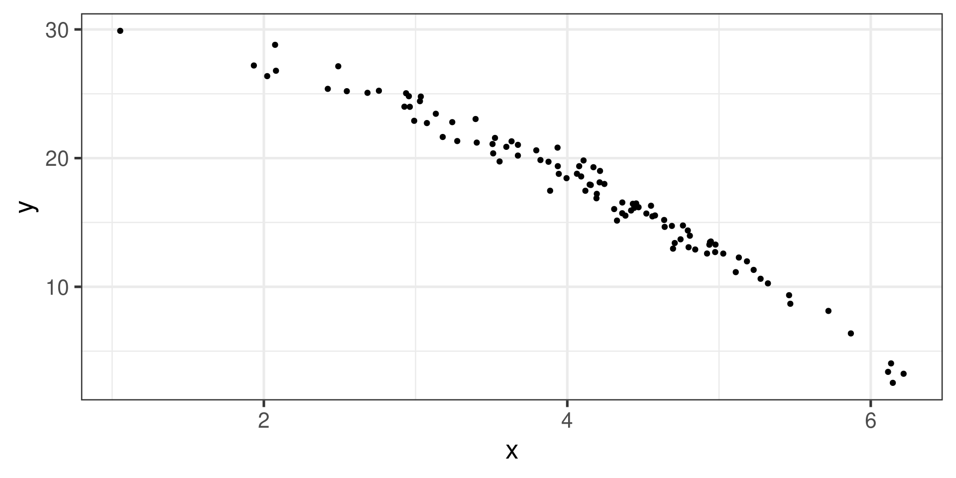
Non-linear association
Non-linear association
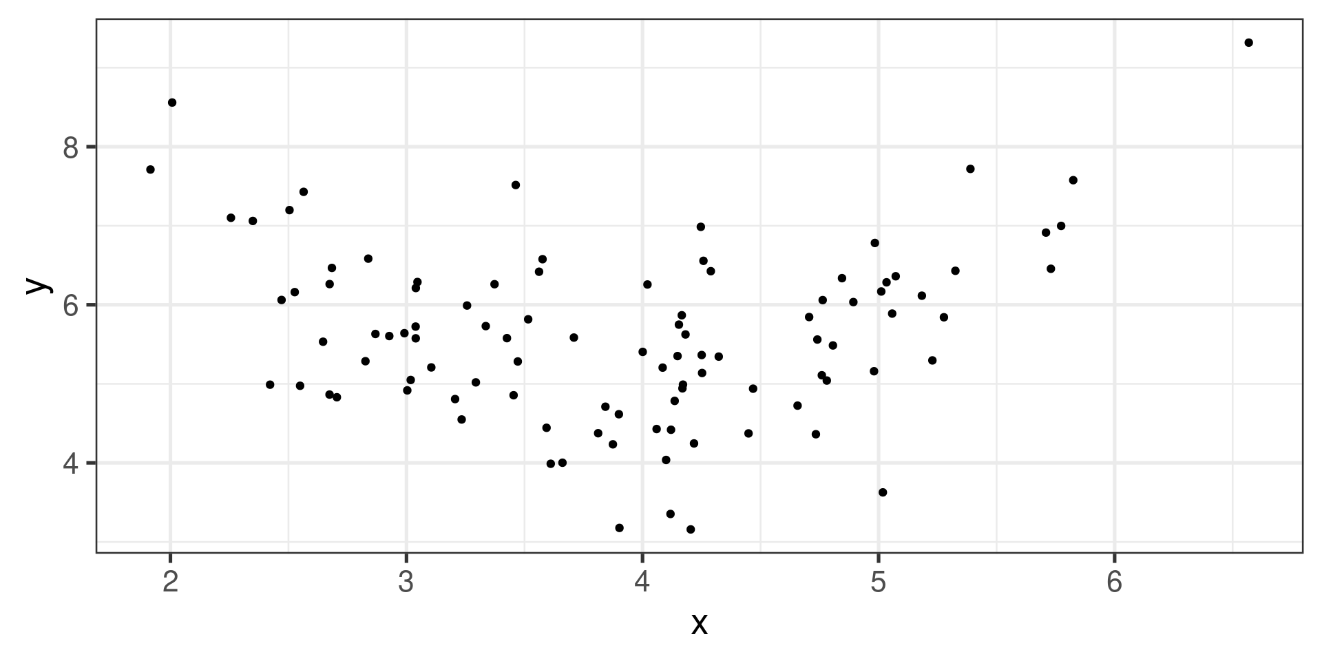
Unclear (very weak linear) association
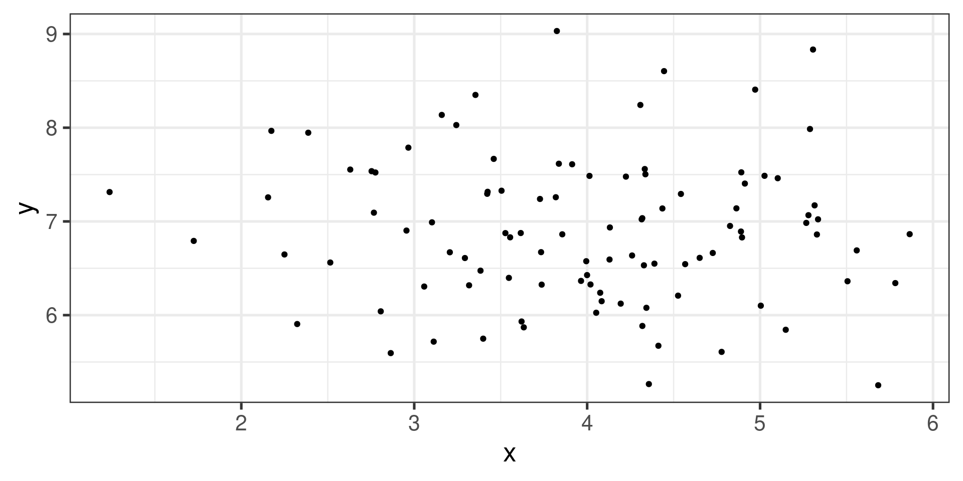
No association, or very weak association
\(\overline{x} = 4.0440945\), \(\overline{y} = 8.0651722\)
Not applicable if the scatterplot shows a nonlinear association!
Use only if scatterplot shows a linear association or no clear association
Start by moving data so that the point \((0,0)\) is in the center (subtracting means): \(x - \overline{x}\) and \(y - \overline{y}\).
Multiply together and calculate the mean
To compensate for different spreads, divide by both standard deviations
\[r = \frac{\text{mean}((x - \overline{x})\cdot (y - \overline{y}))}{\sigma_x\cdot\sigma_y}\]
where:
In R: cor(x,y) or cor(y ~ x, data = ...)
Between \(-1\) and \(1\)
\(r > 0\) indicate positive correlation
\(r < 0\) indicates negative correlation
if \(\left\lvert r\right\rvert\) is larger, it means stronger correlation
Population correlation coefficient is denoted \(\rho\) (rho).
\(H_0\): There is no correlation (\(\rho = 0\)).
\(H_A\): There is a (positive, negative) correlation (\(\rho \neq (>, <) 0\)).
We have a sample with correlation coefficient \(r\), we want to know if it is a strong enough evidence to reject \(H_0\).
Permutation test!
We can also calculate a t-statistic:
\[t = r\sqrt{\frac{n-2}{1-r^2}}\]
This has t-distribution with \(n-2\) degrees of freedom.
What now?
Find a mathematical model for the association:
\[y = ax + b\]
Data is scattered, so the relation will actually be
\[ y = ax + b + \text{ "noise"} \]
Official name for the “noise” is residuals.
predicted value of \(y\): \[\widehat{y} = ax + b\]
actual or observed value of \(y\): \[y = \widehat{y} + e\]
\(e = y - \widehat{y}\) is the residual
The population model: \[\widehat{y} = \beta_0 + \beta_1 x\]
The estimate based on the sample: \[\widehat{y} = b_0 + b_1 x\]
\(\widehat{y}\) is the predicted value
\(b_0\) is the point estimate of \(\beta_0\): the intercept.
\(b_1\) is the point estimate of \(\beta_1\): the rate of change.
The population model: \[y = \beta_0 + \beta_1 x + \varepsilon\]
The estimate based on the sample: \[y = b_0 + b_1 x + e\]
\(e\) is the residual (noise)
\(\varepsilon\) is the random variable representing the residuals
\[b_1 = r\frac{s_y}{s_x}\]
and
\[b_0 = \overline{y} - b_1\overline{x}\]
Usually done by computer
lm(RFFT ~ Age, data = prevend.samp)
Call:
lm(formula = RFFT ~ Age, data = prevend.samp)
Coefficients:
(Intercept) Age
137.550 -1.261 The least squares line can be written as \[ \widehat{\text{RFFT}} = 137.55 - 1.26 (\text{Age}) \]