slides – Math 132B

Categorical variables

Two or more levels
Proportion of one of the levels (success)
Proportions of all the levels (distribution)
Comparison of proportions or distributions between groups (two categorical variables)

Advanced melanoma

Advanced melanoma is an aggressive form of skin cancer that until recently was almost uniformly fatal.

Research is being conducted on therapies that might trigger an immune response to the cancer and cause the melanoma to stop progressing or disappear entirely.

In a study where 52 patients were treated concurrently with two new therapies, nivolumab and ipilimumab, 21 had an immune response. (Wolchok, et. al. NEJM (2013) 369(2): 122-33.)

Advanced melanoma…

Questions that can be addressed with inference…

What is the estimated population probability of immune response following concurrent therapy with nivolumab and ipilimumab?
What is the 95% confidence interval for the estimated population probability of immune response following concurrent therapy with nivolumab and ipilimumab?
In previous studies, the proportion of patients responding to one of these agents was 30% or less. Do these results suggest that the probability of response to concurrent therapy is better than 0.30?

Inference for binomial proportions

The melanoma data are binomial data, with success defined as experiencing an immune response.

Inference is made about the population parameter $𝑝$ , the probability of success in the population.
The estimate of $𝑝$ from the observed sample is $ˆ 𝑝 = 𝑥 / 𝑛$ , where $𝑥$ is the observed number of successes.
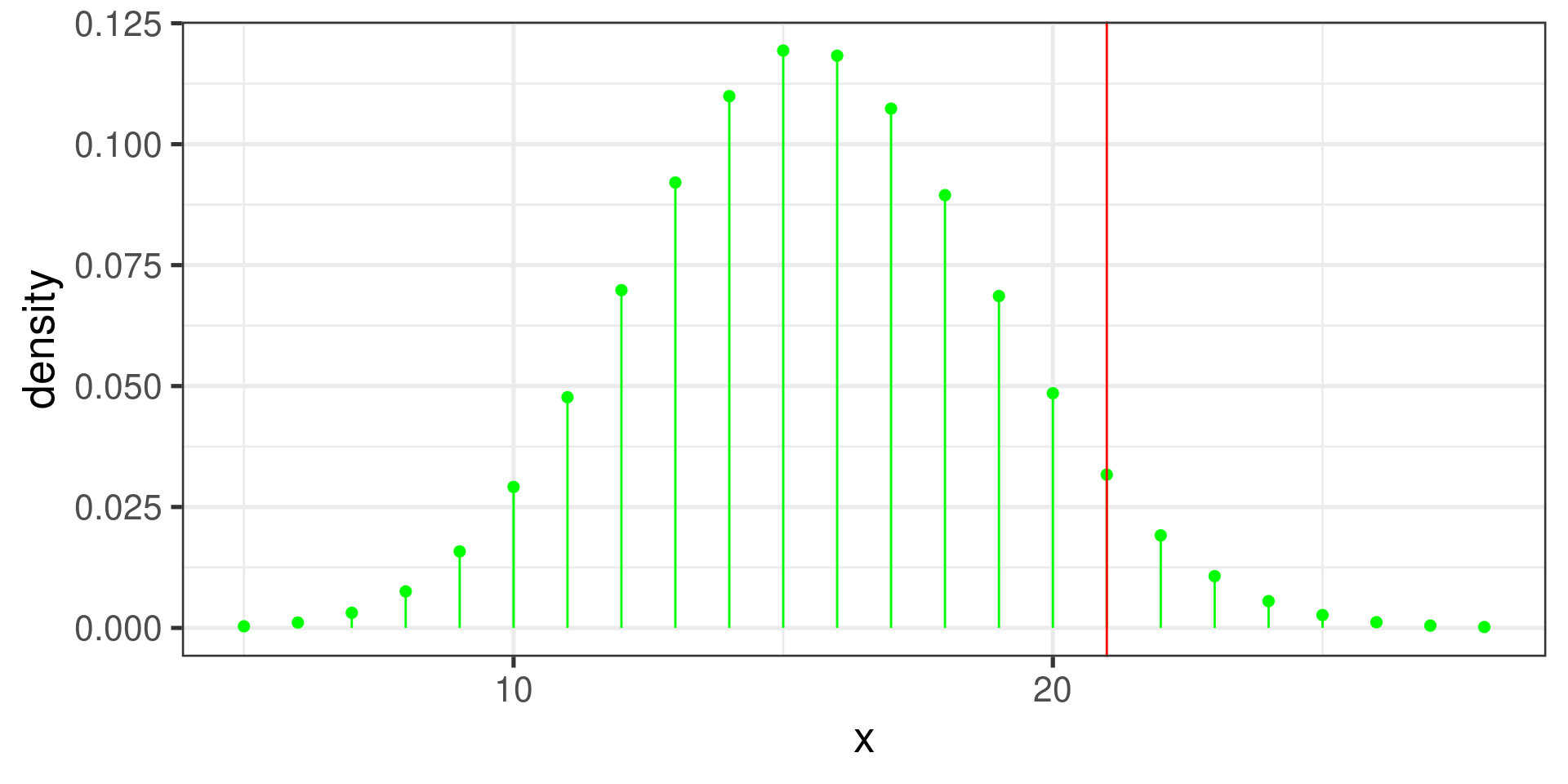
The test statistic can be $𝑥 = 𝑛 ˆ 𝑝$ (the number of successes) which has $B i n o m (𝑛, 𝑝)$ distribution.
We can also use $ˆ 𝑝$ as the test statistic. We know that $𝑛 ˆ 𝑝 \sim B i n o m (𝑛, 𝑝)$ .

Sampling distribution

We could use binomial distribution as sampling distribution

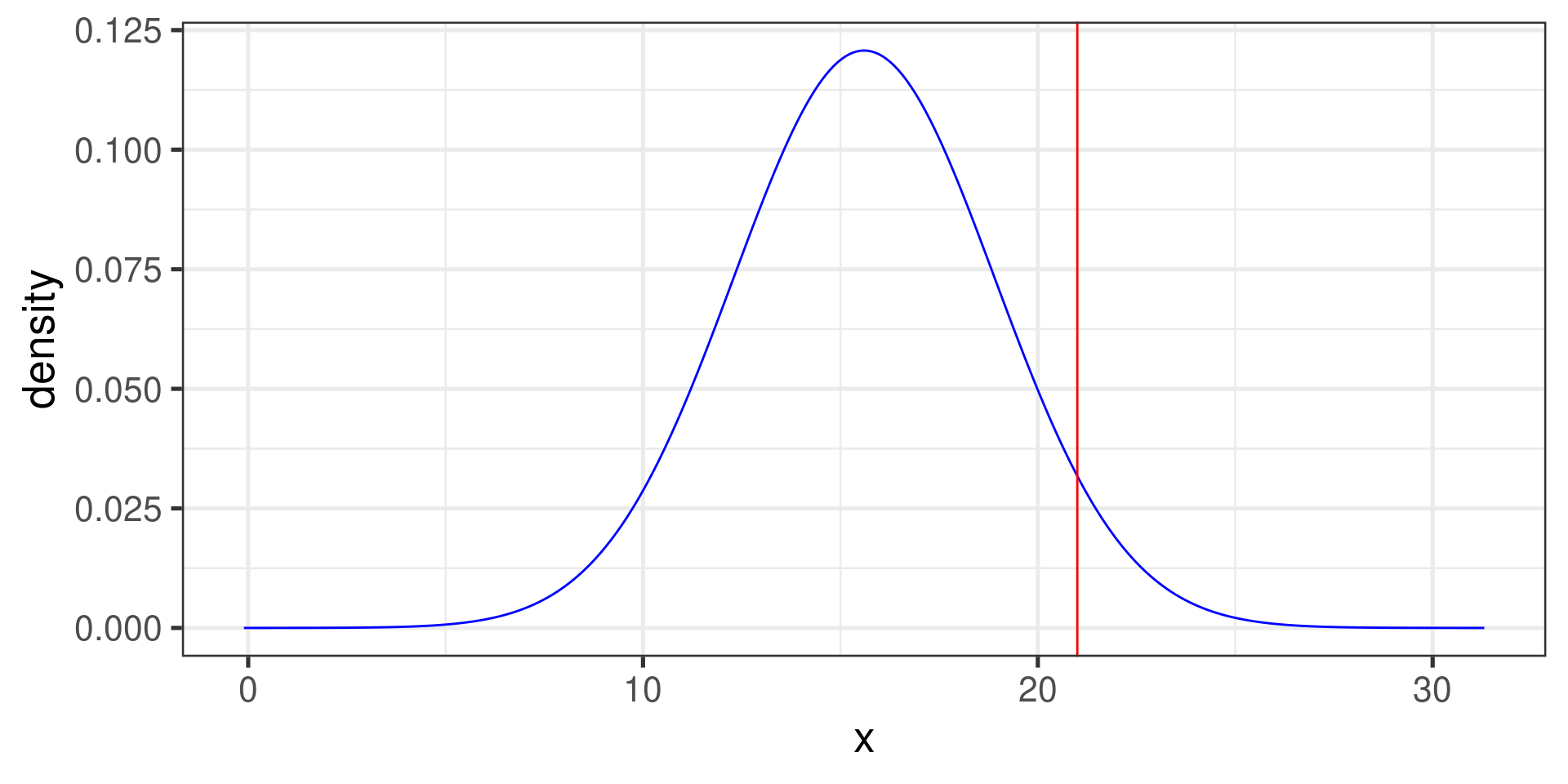
Hard to work with when samples are large.
Discrete distribution, makes finding quantiles tricky.

Under certain assumptions, binomial distribution can be approximated by normal distribution.

Expected number of successes and failures must be large enough
Use $𝜇 = 𝑛 \cdot 𝑝$ and $𝜎 = \sqrt 𝑛 \cdot 𝑝 \cdot (1 - 𝑝)$ .

Sampling distribution

Number of successes: $𝑥 \sim N o r m (𝑛 𝑝, \sqrt 𝑛 𝑝 𝑞)$
Proportion of successes: $ˆ 𝑝 = 𝑥 𝑛$ , so we divide by $𝑛$ and get $ˆ 𝑝 \sim N o r m (𝑝, \sqrt 𝑝 𝑞 𝑛)$

Assumptions for using the normal distribution

The sampling distribution of $ˆ 𝑝$ is approximately normal when

The sample observations are independent, and
At least 10 successes and 10 failures are expected in the sample: $𝑛 𝑝 \geq 10$ and $𝑛 (1 - 𝑝) \geq 10$ . (This condition is commonly referred to as the success-failure condition.)

Under these conditions, $ˆ 𝑝$ is approximately normally distributed with mean $𝑝$ and standard error $\sqrt 𝑝 (1 - 𝑝) 𝑛$ .

When computing an interval estimate, $𝑝$ is unknown, so we substitute $ˆ 𝑝$ for $𝑝$ when using the standard error of $ˆ 𝑝$ .

Inference with normal approximation

In the context of calculating CIs, substitute $ˆ 𝑝$ for $𝑝$ .

An approximate two-sided confidence interval for $𝑝$ is given by $ˆ 𝑝 \pm 𝑧 ⋆ \sqrt ˆ 𝑝 (1 - ˆ 𝑝) 𝑛 .$

Example: $𝑥 = 21$ , $𝑛 = 52$ , find 95% CI for $𝑝$ .

prop.test(x = 21, n = 52, conf.level = 0.95)$conf.int

[1] 0.2731269 0.5487141
attr(,"conf.level")
[1] 0.95

Inference with normal approximation

In the context of hypothesis testing, substitute $𝑝 0$ for $𝑝$ .

The test statistic $𝑧$ for the null hypothesis $𝐻 0 : 𝑝 = 𝑝 0$ is $𝑧 = ˆ 𝑝 - 𝑝 0 \sqrt (𝑝 0) (1 - 𝑝 0) 𝑛$

Example: $𝑥 = 21$ , $𝑛 = 52$ , test $𝐻 0 : 𝑝 = 0.30$ , $𝐻 𝐴 : 𝑝 > 0.30$ .

prop.test(x = 21, n = 52, p = 0.30, alternative = "greater")


    1-sample proportions test with continuity correction

data:  21 out of 52
X-squared = 2.1987, df = 1, p-value = 0.06906
alternative hypothesis: true p is greater than 0.3
95 percent confidence interval:
 0.2906582 1.0000000
sample estimates:
        p 
0.4038462

Inference with normal approximation

Exact inference for binomial data

Using the binomial distribution:

p-value is $𝑃 (𝑥 \geq 21 | 𝑝 = 0.30)$

pbinom(20, size = 52, p = 0.30, lower.tail = FALSE)

[1] 0.07167176

The exact binomial test:

binom.test(x = 21, n = 52, p = 0.30, alternative = "greater")




data:  21 out of 52
number of successes = 21, number of trials = 52, p-value = 0.07167
alternative hypothesis: true probability of success is greater than 0.3
95 percent confidence interval:
 0.2889045 1.0000000
sample estimates:
probability of success 
             0.4038462

Exact inference for binomial data

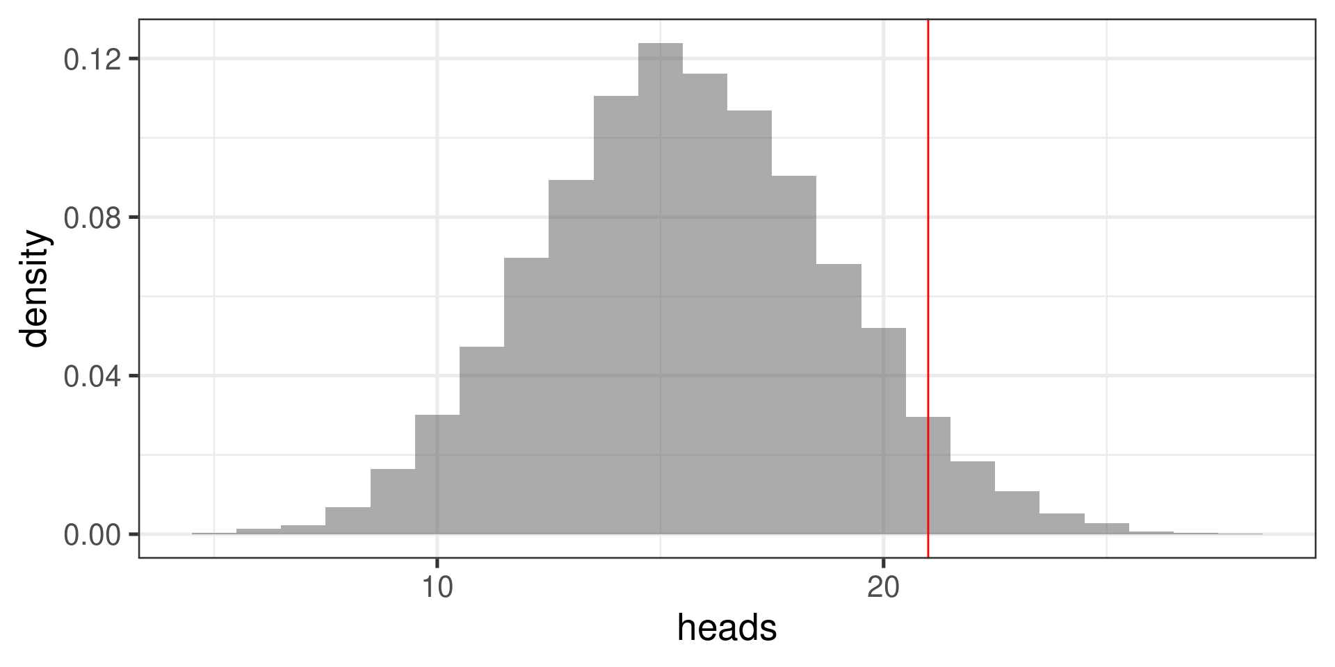
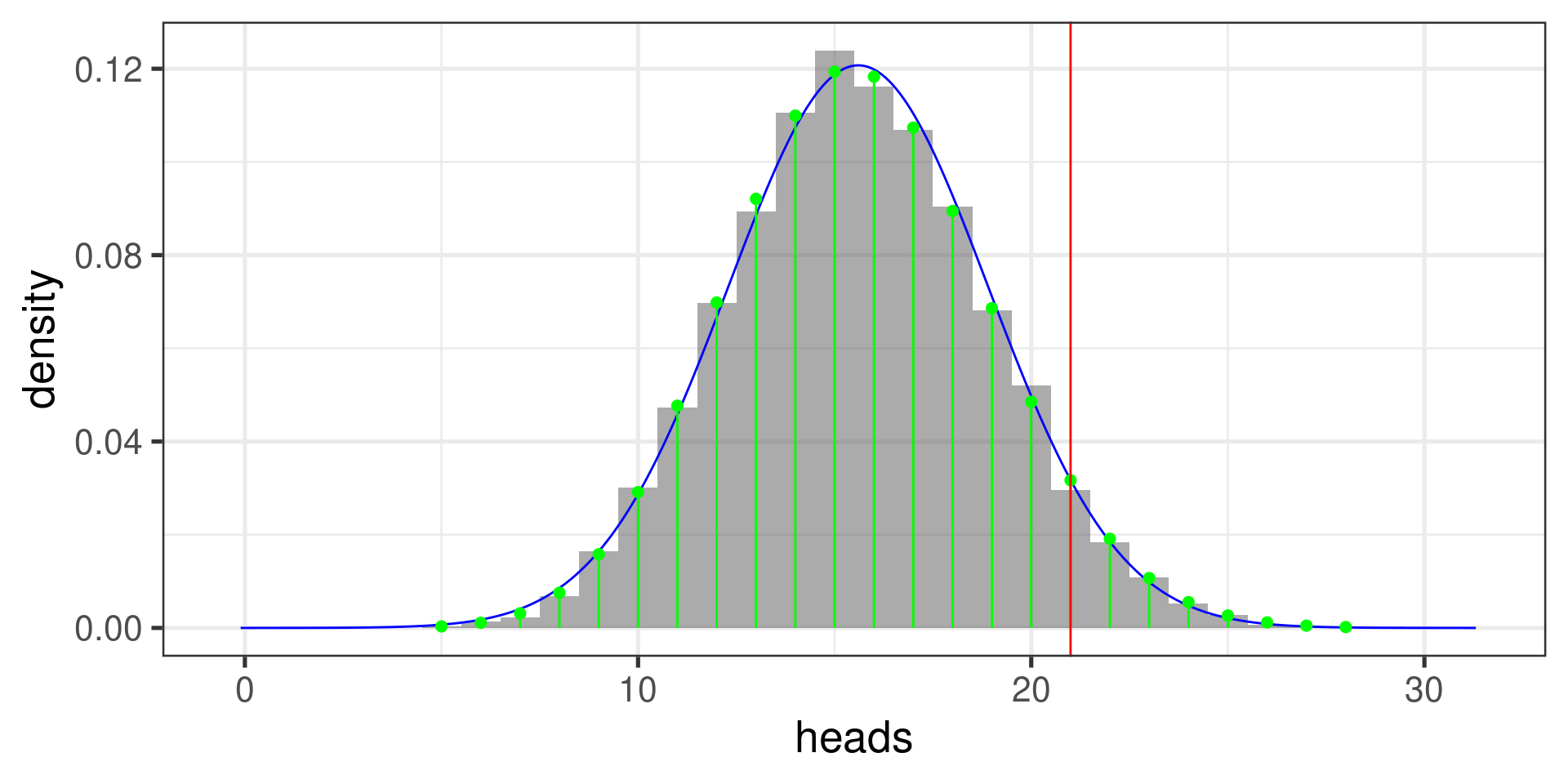
Another option: simulation

do(10000) * rflip(52, prob = 0.30) -> sims
prop(~(heads >= 21), data = sims)

prop_TRUE 
    0.068

Another option: simulation

Comparison of all three

Inference for the difference of two proportions

Difference of two independent normally distributed variables is normally distributed.
The mean is the difference of the two means.
The variance is the sum of the two variances.
The standard deviation is the square root of the sum of the two variances.
The normal model can be applied to $ˆ 𝑝 1 - ˆ 𝑝 2$ if
1. The two samples are independent, the observations in each sample are independent, and
2. At least 10 successes and 10 failures are expected in each sample.

Inference for the difference of two proportions

The standard error of the difference in sample proportions is $\sqrt 𝑝 1 (1 - 𝑝 1) 𝑛 1 + 𝑝 2 (1 - 𝑝 2) 𝑛 2$

In hypothesis testing, the following estimate of $𝑝$ is used to compute the standard error: $ˆ 𝑝 = 𝑛 1 ˆ 𝑝 1 + 𝑛 2 ˆ 𝑝 2 𝑛 1 + 𝑛 2 = 𝑥 1 + 𝑥 2 𝑛 1 + 𝑛 2$

Use this for both $𝑝 1$ and $𝑝 2$ .

Are metal bands used for tagging harmful to penguins?

Researchers (Saraux at al., 2011) wanted to know whether metal bands used for tagging penguins are harmful. They selected a random sample of 100 penguins, tagged them with RFID chips, and tagged 50 of them with metal bands. After about 4 years, they checked how many penguins in each group survived.

Data

ABCDEFGHIJ0123456789

group <chr>	survived <lgl>
band	FALSE
band	FALSE
band	FALSE
band	FALSE
band	FALSE
band	TRUE
band	FALSE
band	FALSE
band	FALSE
band	FALSE

Results

        group
survived band control
   TRUE    16      31
   FALSE   34      19

The same with proportions:

        group
survived band control
   TRUE  0.32    0.62
   FALSE 0.68    0.38

What does it mean?