Math 132B
Class 28
Categorical variables
-
Single categorical variable:
-
Two levels:
Single proportion
-
More than two levels:
Goodness of fit test
-
-
Two categorical variables:
-
Both with two levels:
Difference of proportions
-
More than two levels:
Independence test
-
Are metal bands used for tagging harmful to penguins?
Researchers (Saraux at al., 2011) wanted to know whether metal bands used for tagging penguins are harmful. They selected a random sample of 100 penguins, tagged them with RFID chips, and tagged 50 of them with metal bands. After about 4 years, they checked how many penguins in each group survived.
Data
Results
        group
survived band control
   TRUE    16      31
   FALSE   34      19
group
survived band control
TRUE 0.32 0.62
FALSE 0.68 0.38\[SE = \sqrt{\dfrac{p_1(1 - p_1)}{n_1} + \dfrac{p_2(1 - p_2)}{n_2}} \]
\[\hat{p} = \dfrac{n_1\hat{p}_1 + n_2\hat{p}_2}{n_1 + n_2} = \dfrac{x_1 + x_2}{n_1 + n_2} \]
Goodness of fit
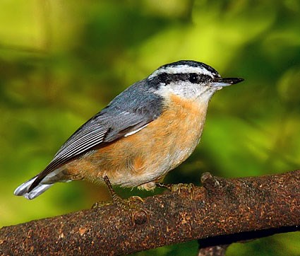
Red-breasted nuthatch (Sitta canadensis)
These insect eating birds search bark furrows for hidden prey.
Do these birds prefer certain kinds of trees?
Mannan and Meslow (1984) studied red-breasted nuthatch foraging behavior in a managed forest in Oregon. In the forest, 54% of the canopy volume was Douglas fir, 40% was ponderosa pine, 5% was grand fir, and 1% was western larch. They made 156 observations of foraging by red-breasted nuthatches; 70 observations (45% of the total) in Douglas fir, 79 (51%) in ponderosa pine, 3 (2%) in grand fir, and 4 (3%) in western larch.
Do these data show a preference for some species of trees?
Goodness of fit
We have a single categorical variable with 3 or more levels.
We are asking whether the categorical variable follows certain specific distribution.
\(H_0: p_{DF} = .54 \text{ and } p_{PP} = .4 \text{ and } p_{GF} = .05 \text{ and } p_{WL} = .01\)
\(H_A:\) the tree choices do not follow this distribution.
Categorical variable: we can do a simulation
What do we use as a test statistic?
Comparing observed with expected
Observed counts: 70, 79, 3, 4
-
Expected counts:
- 54% of 156 \({} = 84.24\)
- 40% of 156 \({} = 62.4\)
- 5% of 156 \({} = 7.8\)
- 1% of 156 \({} = 1.56\)
Discrepancy
\[\begin{alignat}{3} && \text{Observed} &- \text{Expected} &\\[1.2ex] &\text{Douglas fir: } & 70 &- 84.24 &=& &\quad\class{fragment}{-14.24}\\[1.2ex] &\text{Ponderosa pine: } & 79 &- 62.40 &=& &\class{fragment}{16.60}\\[1.2ex] &\text{Grand fir: } & 3 &- 7.80 &=& &\class{fragment}{-4.80}\\[1.2ex] &\text{Western larch: } & 4 &- 1.56 &=& &\class{fragment}{2.44}\\[1.2ex] \end{alignat}\]
Two problems
- We need to combine all four numbers together to get one value.
- Some are negative while some are positive.
- The numbers are not directly comparable: they come from different totals!
Solution
-
Convert them to z-scores
\(\displaystyle z = \frac{x - \mu}{\sigma} = \frac{\text{Observed} - \text{Expected}}{\sqrt{\text{Expected}}}\)
-
Square them and add the squares.
\(\displaystyle \sum z^2 = \sum \left(\frac{x - \mu}{\sigma}\right)^2 = \sum \left(\frac{\text{Observed} - \text{Expected}}{\sqrt{\text{Expected}}}\right)^2\)
\(\chi^2\) statistic:
\[\chi^2 = \sum \frac{\left(\text{Observed} - \text{Expected}\right)^2}{\text{Expected}}\]
\[\chi^2 = \frac{(70 - 84.24)^2}{84.24} + \frac{(79 - 62.4)^2}{62.4} + \frac{(3 - 7.8)^2}{7.8} + \frac{(4 - 1.56)^2}{1.56} \]
\[= \frac{(-14.24)^2}{84.24} + \frac{(16.6)^2}{62.4} + \frac{(-4.8)^2}{7.8} + \frac{(2.44)^2}{1.56} \]
\[\chi^2 = 13.59 \]
Simulation
Is \(\chi^2 = 13.59\) small or large?
\(\chi^2\) table
